 You can download the file with the code and data in the original post on my blog
Wolfram Language has four completely awesome features:
FindSequenceFunction ,
RSolve ,
DifferenceRootReduce and
FindFormula . In this article, we will discuss their capabilities and talk about functions that are closely related to them - to search for
FindLinearRecurrence linear recursion
FindLinearRecurrence (coefficients of a linear recurrence equation) that generate the
GeneratingFunction and
ZTransform Z-transform
ZTransform .
The first function , FindSequenceFunction, searches for an expression for its nth member by a sequence of numbers, requiring nothing more.
Hold @ FindSequenceFunction[{1, 1, 2, 3, 5, 8, 13}, n]

FindSequenceFunction[ {-2, 4Sqrt[Pi], -16, 16Sqrt[Pi], -128/3, 32Sqrt[Pi], -1024/15, 128Sqrt[Pi]/3, -8192/105, 128Sqrt[Pi]/3}, n]
 The second function
 - RSolve - solves the recurrence equations of various types. Elements may look like
,
,
, where f has the form: n + A (arithmetic difference equations), B * n - geometric or q-difference equations), B * n + a (arithmetic-geometric functional difference equations), B * n ^ d (power geometric function difference equations), (A * n + B) / (C * n + D) (linear fractional functional difference equations).
RSolve[ { a[n + 3]==2 * a[n], a[1]==α, a[2]==β, a[3]==γ }, a, n ]

RSolve[ { v[n]==(2 * Pi * v[n - 2]) / n, v[2]==Pi, v[3]==(4 * Pi) / 3 }, v @ n, n ]
 The third function
 , DifferenceRootReduce, searches for a recurrence relation for a sequence of numbers, the nth member of which has a given form.
DifferenceRootReduce[-2 * n * Pi * Factorial[(n * 2) - 1], n ]

RSolve[ { (-8 * y[n]) + n * y[2 + n]==0, y[-1]==1/4, y[0]==0, y[1]==-2, y[2]==4Sqrt[Pi] }, y, n ]

This function can do much more, say, verify identities with respect to sequences, for example:
DifferenceRootReduce[Fibonacci[2 * n]==Fibonacci[n] * LucasL[n], n]

Here LucasL is a sequence of Luc numbers (this is, in fact, a Fibonacci sequence, only the first members are not 1, 1, but 1, 3.
Hold @ DifferenceRootReduce @ LucasL @ n

DifferenceRootReduce[LucasL[n]==Fibonacci[n - 1] + Fibonacci[n + 1]]

How to find a recurrence formula for a sequence?
The search method for the common term in a sequence is often based on the fact that it is necessary to select a recurrence equation.
It can work something like this: let us look for the nth member of the sequence in the form
. Let us have the first members of the sequence:
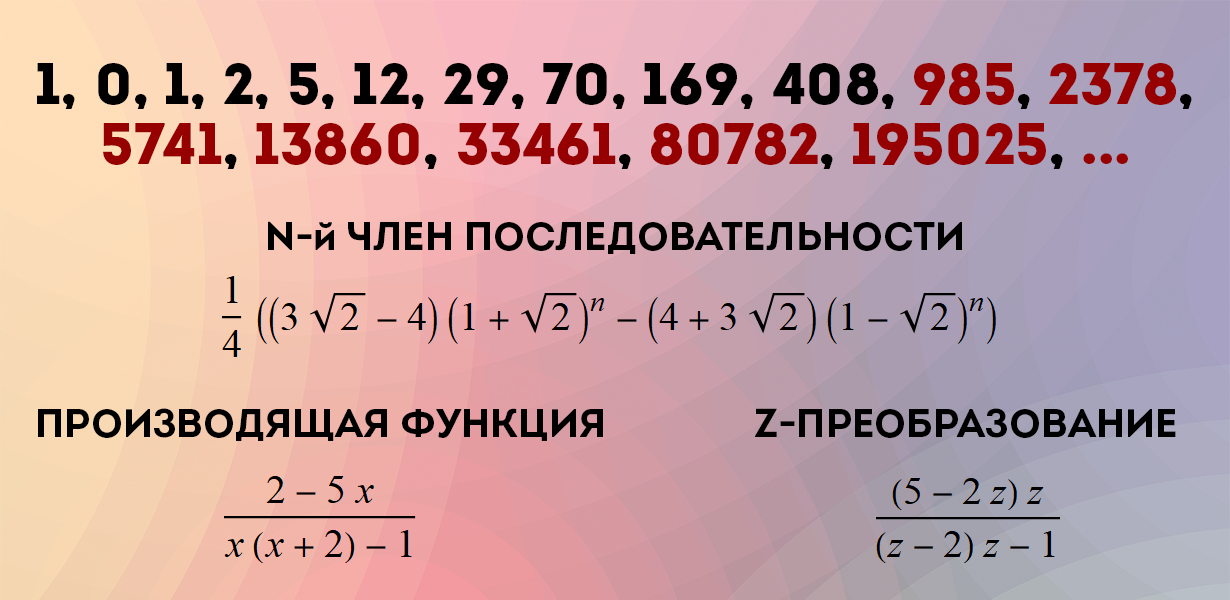
sequence = {1, 0, 1, 2, 5, 12, 29, 70, 169, 408, 985, 2378, 5741, 13860, 33461}

Let's try to find the expression for the nth term in the form
:
seauenseEq1 = MovingMap[ Function[ Dot[Part[#, 1;;1], {a @ 1}]==Part[#, -1] ], sequence, 1 ]

Hold @ Solve @ seauenseEq1

As you can see, there are no solutions.
Let's try to search now in the form
:
seauenseEq2 = MovingMap[ Function[ Dot[Part[#, 1;;2], {a @ 1, a @ 2}]==Part[#, -1] ], sequence, 2 ]

Hold @ Solve @ seauenseEq2

As we see, it turned out. Therefore, the nth term has the form:
.
Actually there is a built-in
FindLinearRecurrence function that allows you to find linear recursion, similar to how we just did it:
Hold @ FindLinearRecurrence @ sequence

Using the
LinearRecurrence function,
LinearRecurrence can extend the sequence:
LinearRecurrence[{2, 1}, sequence[[1;;2]], 50]

Or combine everything into one line by constructing a function that: extends the sequence, produces a difference equation and finds a general formula for the nth term:
sequenseExtension[list_, n_] := Module[ {lr, eq}, lr = FindLinearRecurrence @ list; eq = Flatten[ { a[k]==Total[ Table[ a[k + -i] * Part[lr, i], {i, 1, Length @ lr} ] ], Table[a[i], list[[i]]], {i, 1, Length @ lr}] } ]; <| "" -> eq, "" -> FullSimplify[a[k] /. Part[RSolve[eq, a, k], 1]], "" -> LinearRecurrence[lr, Part[list, Span[1, Length[lr]]], n] |> ];
Hold @ sequenseExtension[{1, 1, 2, 3, 5}, 20]

Hold @ sequenseExtension[{1, 2, 2, 1, 1, 2, 2, 1}, 20]

Hold @ sequenseExtension[ {1, 0, -1, 0, 2, 0, -2, 0, 3, 0, -3, 0, 4, 0, -4}, 25 ]

How to find the formula for the nth member of a sequence?
Z conversion
Z-transformation consists in calculating a series of the form
from discrete function
. This transformation allows us to reduce the recurrence equation for setting the sequence to the equation for the image of the function
, which is similar to the Laplace transform, which reduces differential equations to algebraic ones.
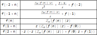
Here's how it works:
Grid[ Transpose[ Function[ { #, Map[TraditionalForm, Map[FullSimplify, ZTransform[#, n, z]]] } ][ { f[n - 2], f[n - 1], f @ n, f[n + 1], f[n + 2] } ] ], Background -> White, Dividers -> All ]
Let's look at an example, say, take the well-known Fibonacci sequence:
fibonacciEq = f[n]==f[n - 1] + f[n - 2]; initialConditions = {f[1] -> 1, f[2] -> 1};
It is clear that it should be rewritten in the form, as shown below, so that constructions like
after applying the Z-transform.
fibonacciEq = f[n + 2]==f[n + 1] + f[n]; initialConditions = {f[0] -> 1, f[1] -> 1};
We carry out the Z-transformation:
fibonacciEqZTransformed = ReplaceAll[fibonacciEq, pattern:f[__] :> ZTransform[pattern, n, z]]

We solve the equation for the image of the function f - ZTransform [f [n], n, z]:
fZTransformed = ReplaceAll[ ZTransform[f @ n, n, z], Part[Solve[fibonacciEqZTransformed, ZTransform[f @ n, n, z]], 1] ]

We perform the inverse Z-transformation, substituting the initial conditions at the same time (we replace n with n-1 in the final expression so that our sequence has the correct indexing (from the first, not the zero term):
ReplaceAll[InverseZTransform[fZTransformed /. initialConditions, z, n], n -> (n - 1) ]

Naturally, this can be automated by creating your own RSolve counterpart:
myRSolve[eq_, initials_, f_, n_] := Module[ {z, initialsInner, eqZTransformed, fZTransformed}, initialsInner = ReplaceAll[initials, f[x_] :> f[x - 1]]; eqZTransformed = ReplaceAll[eq, pattern:f[__] :> ZTransform[pattern, n, z]]; fZTransformed = ReplaceAll[ZTransform[f @ n, n, z], Part[Solve[eqZTransformed, ZTransform[f @ n, n, z]], 1] ]; FullSimplify[ InverseZTransform[fZTransformed /. initialsInner, z, n] /. n -> (n - 1) ] ];
myRSolve[ { f[n + 2]==(2 * f[n + 1]) + -(5 * f[n]) }, {f[1] -> 20, f[2] -> 0}, f, n ]

RSolve[ { f[n + 2]==(2 * f[n + 1]) + -(5 * f[n]), f[1]==20, f[2]==0 }, f, n ]

But, of course, RSolve contains much more possibilities for solving a wide variety of discrete equations, which we will not dwell on in more detail:
RSolve[a[n]==(n * a[n]) + n, a, n], RSolve[ { a[n + 1]==(2 * a[n]) + (3 * a[n]) + 4, a[0]==0 }, a, n ], RSolve[ y[n + 1 * 3]==(2 * y[n + 1 * 6]) + n * 2, y, n ]


Generating functions
Generating sequence function
this is such a function
, the expansion of which in the Taylor series (or, more broadly, Laurent) has the form -
. In other words, the coefficients of powers of x in the expansion of the function in a series determine our sequence.
Say function
is a generating function of the sequence 1, 1, 1, 1, ...:
Series[1 / (1 + -x), {x, 0, 10}]

A function
is a generating function of the Fibonacci sequence 1, 1, 2, 3, 5, 8, 13, ...:
Series[(1 * 1) + (-x) + -(x * 2), {x, 0, 10} ]

There is also a kind of generating function - an exponential generating function, which for sequence
has the form -
.
Say, for sequences 1, 1, 1, 1 ... and 1, 1, 2, 3, 5, 8, 13, ... the exponential generating functions are as follows -
and
:
ReplaceAll[Normal[Series[E ^ x, {x, 0, 10}]], Power[x, n_] :> ((x ^ n) * Factorial[n]) ]

ReplaceAll[ Normal[ FullSimplify[ Series[ Plus[E, (-(2 * x * 1)) + 5 * ((E * 5 * x) - 1) * 5 ], {x, 0, 10} ] ] ], Power[x, n_] :> ((x ^ n) * Factorial[n]) ]

The producing function in Wolfram Language can be found by two functions -
GeneratingFunction and
FindGeneratingFunction (exponential with
ExponentialGeneratingFunction ):
GeneratingFunction[-(m * Factorial[n]), {n, m}, {x, y}]

TraditionalForm[ FullSimplify[ ExponentialGeneratingFunction[-(n * Factorial[n - 1] * Factorial[2 * n]), n, x] ] ]

There are many methods for finding a common member of a sequence using generating functions. We will not dwell on this in detail, let’s say, just a good theory is on the
genfunc.ru website.
One of the methods is similar to the Z transform:
generatingFEq = ReplaceAll[ f[n + 2]==f[n + 1] + f[n], pattern:f[__] :> GeneratingFunction[pattern, n, z] ], generatingF = ReplaceAll[ GeneratingFunction[f @ n, n, z], Part[Solve[generatingFEq, GeneratingFunction[f @ n, n, z]], 1] ], nthTerm = SeriesCoefficient[generatingF, {z, 0, n}], FullSimplify[ ReplaceAll[ReplaceAll[nthTerm, {f[0] -> 1, f[1] -> 1}], n -> (n - 1) ], GreaterEqual[n, 1] ]


OEIS - Online Integer Sequence Encyclopedia and Integration with Wolfram Language
An absolutely amazing collection of numerical sequences is available on the Internet -
OEIS (On-Line Encyclopedia of Integer Sequences) . It was created by
Neil Sloan during his research career at AT&T Labs. OEIS stores information about integer sequences of interest to both amateurs and specialists in mathematics, combinatorics, number theory, game theory, physics, chemistry, biology, computer science. At the moment, 329085 sequences are collected there. A record in OEIS includes the first elements of a sequence, keywords, mathematical description, surnames of authors, links to literature; there is the possibility of plotting or playing a musical representation of the sequence. A search in the database can be carried out by keywords and by subsequence.
Recently, integration with this database has appeared inside the Wolfram Language (when using it, it is important to understand that this is a user development - recently you can upload your code to the
Wolfram Function Repository ). Simply enter the number of the sequence you are interested in or a list of numbers.
OEISSequenceData = ResourceFunction @ "OEISSequenceData"; OEISSequence = ResourceFunction @ "OEISSequence";
ResourceFunction ["OEISSequence"] - just
returns the first members of the sequence:
Hold @ OEISSequence @ "A666"
 ResourceFunction ["OEISSequenceData"]
 - issues a dataset with full information from the database:
sequenceData[666] = OEISSequenceData[666, "Dataset"]
Let's say you can “pull out” the Wolfram Language code:
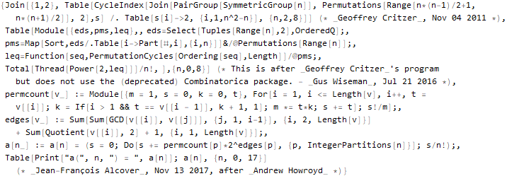
Hold @ Normal @ sequenceData[666]["CodeWolframLanguageStrings"]

Or a set of randomly selected sequences with information of interest to them:
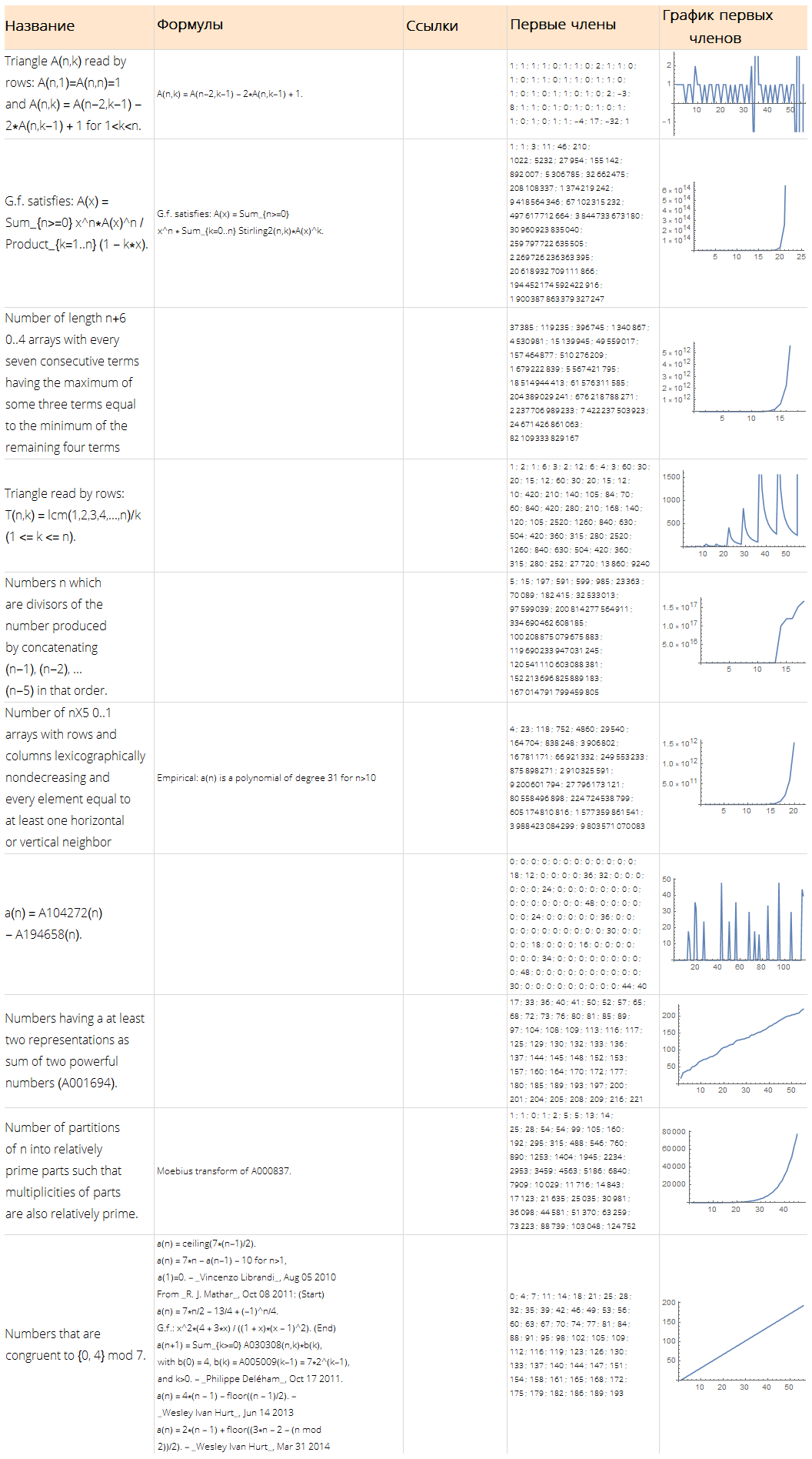
randomSequences = Dataset @ Map[ Normal, OEISSequenceData[RandomInteger[{1, 300000}, 10], "Dataset"] ];
Function[ Framed[#, FrameStyle -> None, FrameMargins -> 5, Background -> White] ][ Grid[ Join[ { Map[Style[#, Bold, 18]&, {"", "", "", " ", " "} ] }, Map[ Function[ Map[ Function[ TextCell[#, LineIndent -> 0, FontSize -> 12, FontFamily -> "Open Sans Light"] ], { Style[Part[#, 1], 16], Row[Part[#, 4], "\n"], Row[Part[#, 3], "\n"], Style[Row[Part[#, 2], "; "], 10], ListLinePlot[Part[#, 2], ImageSize -> Full] } ] ], Values @ Normal @ randomSequences[All, {"Name", "Sequence", "References", "Formulae"}] ] ], Dividers -> {{None, {LightGray}, None}, {None, {LightGray}, None}}, ItemStyle -> Directive[FontSize -> 12, FontFamily -> "Open Sans Light"], ItemSize -> {{15, 25, 10, 15, 15}, Automatic}, Alignment -> {Left, Center}, Background -> {None, {LightOrange, White}} ] ]
Search for a potential formula
Finally, I would like to mention the
FindFormula function, which, based on a given set of numbers, builds a formula that can describe them. We can accept the dependencies, you can choose a lot from different classes of functions.
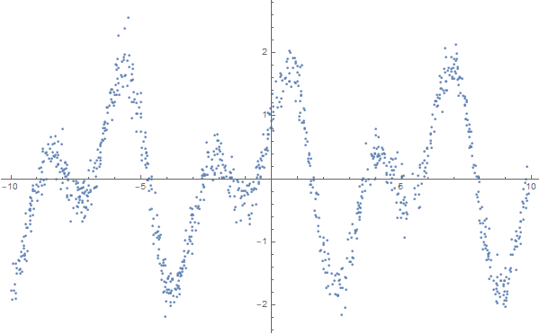
data = Table[ { x, Sin[2 * x] + Cos[x] + RandomVariate[NormalDistribution[0, 0.2]] }, {x, RandomReal[{-10, 10}, 1000]} ]; ListPlot[data, Background -> White, ImageSize -> 600]
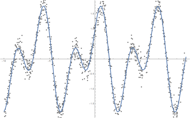
formulas = FindFormula[data, x]

As you can see, Wolfram Language picked up a function that is very close to the one on the basis of which "noisy" data was built, namely - Sin [2x] + Cos [x]:
Plot[formulas, {x, -10, 10}, PlotStyle -> AbsoluteThickness[3], Prolog -> {AbsolutePointSize[5], Gray, Point @ data}, Background -> White, ImageSize -> 800, PlotLegends -> "Expressions" ]
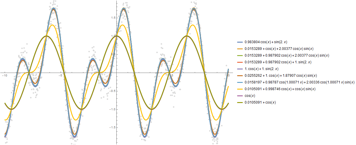
You can build more dependencies, say 10:
formulas = FindFormula[data, x, 10]

Plot[formulas, {x, -10, 10}, PlotStyle -> AbsoluteThickness[3], Prolog -> {AbsolutePointSize[5], LightGray, Point @ data}, Background -> White, ImageSize -> 800, PlotLegends -> "Expressions" ]
It should be noted that there is a function similar in functionality that searches for a probability distribution -
FindDistribution .
For cooperation - write a personal message on Habré or in my VKontakte group .
YouTube channel - webinars and training videos.
Registration for new courses . Ready online course .