R-
dplyrおよび
data.tableデータを操作するための2つの優れたパッケージがあります。 各パッケージには独自の長所があります。
dplyrエレガントで自然言語に似ていますが、
data.table簡潔で、1行で多くのことができます。 さらに、場合によっては、
data.table高速であり(
ここで比較分析を利用でき
ます )、これにより、メモリまたはパフォーマンスに制限がある場合に選択を決定できます。
dplyrと
data.table比較は、
Stack Overflowと
Quoraでも読むことができます。
ここでは、マニュアルと
data.table簡単な説明を、
data.tableについては
こちらを
参照して
dplyr 。 DataScience +で
dplyrを読むこともできます。
最初の部分では、データの使用を開始し、列を選択、削除、および名前変更します。
データから特定の行を選択する
データから一部の行を選択するには、
dplyrの動詞
filterと、正規表現を含む可能性のある条件を使用する必要があります。
data.tableでは、条件のみが必要です。
1つの変数でフィルター
from_dplyr = filter(hospital_spending,State=='CA')
TRUE dropped attributes
複数の変数によるフィルター
from_dplyr = filter(hospital_spending,State=='CA' & Claim.Type!="Hospice") from_data_table = hospital_spending_DT[State=='CA' & Claim.Type!="Hospice"] compare(from_dplyr,from_data_table, allowAll=TRUE)
TRUE dropped attributes
from_dplyr = filter(hospital_spending,State %in% c('CA','MA',"TX")) from_data_table = hospital_spending_DT[State %in% c('CA','MA',"TX")] unique(from_dplyr$State)
CA MA TX
compare(from_dplyr,from_data_table, allowAll=TRUE)
TRUE dropped attributes
データを並べ替える
行を配置するには、
dplyr動詞を使用する必要があります。 これは、1つ以上の変数を使用して実行できます。
desc()ソートするには、例のように
desc()れます。 降順および昇順でソートする例は明らかです。 1つの変数でデータを並べ替えましょう。
昇順
from_dplyr = arrange(hospital_spending, State) from_data_table = setorder(hospital_spending_DT, State) compare(from_dplyr,from_data_table, allowAll=TRUE)
TRUE dropped attributes
降順
from_dplyr = arrange(hospital_spending, desc(State)) from_data_table = setorder(hospital_spending_DT, -State) compare(from_dplyr,from_data_table, allowAll=TRUE)
TRUE dropped attributes
複数の変数で並べ替え
Stateの昇順とEnd_Dateの降順でソートしましょう。
from_dplyr = arrange(hospital_spending, State,desc(End_Date)) from_data_table = setorder(hospital_spending_DT, State,-End_Date) compare(from_dplyr,from_data_table, allowAll=TRUE)
TRUE dropped attributes
列の追加/削除
dplyrは
dplyr mutate()関数を使用して列を追加します。
data.table :=を使用して、参照によって1行で列を追加または変更できます。
from_dplyr = mutate(hospital_spending, diff=Avg.Spending.Per.Episode..State. - Avg.Spending.Per.Episode..Nation.) from_data_table = copy(hospital_spending_DT) from_data_table = from_data_table[,diff := Avg.Spending.Per.Episode..State. - Avg.Spending.Per.Episode..Nation.] compare(from_dplyr,from_data_table, allowAll=TRUE)
TRUE sorted renamed rows dropped row names dropped attributes
from_dplyr = mutate(hospital_spending, diff1=Avg.Spending.Per.Episode..State. - Avg.Spending.Per.Episode..Nation.,diff2=End_Date-Start_Date) from_data_table = copy(hospital_spending_DT) from_data_table = from_data_table[,c("diff1","diff2") := list(Avg.Spending.Per.Episode..State. - Avg.Spending.Per.Episode..Nation.,diff2=End_Date-Start_Date)] compare(from_dplyr,from_data_table, allowAll=TRUE)
TRUE dropped attributes
要約された列情報を取得する
一般化された統計を取得するには、
dplyr summarize()関数を使用できます。
summarize(hospital_spending,mean=mean(Avg.Spending.Per.Episode..Nation.))
mean 8.772727
hospital_spending_DT[,.(mean=mean(Avg.Spending.Per.Episode..Nation.))]
mean 8.772727
summarize(hospital_spending,mean=mean(Avg.Spending.Per.Episode..Nation.), maximum=max(Avg.Spending.Per.Episode..Nation.), minimum=min(Avg.Spending.Per.Episode..Nation.), median=median(Avg.Spending.Per.Episode..Nation.))
mean maximum minimum median 8.77 19 1 8.5
hospital_spending_DT[,.(mean=mean(Avg.Spending.Per.Episode..Nation.), maximum=max(Avg.Spending.Per.Episode..Nation.), minimum=min(Avg.Spending.Per.Episode..Nation.), median=median(Avg.Spending.Per.Episode..Nation.))]
mean maximum minimum median 8.77 19 1 8.5
また、個々のデータの一般的な統計を取得することもできます。
dplyrには
group_by()関数がありますが、
data.tableは
byのみを使用
byます。
head(hospital_spending_DT[,.(mean=mean(Avg.Spending.Per.Episode..Hospital.)),by=.(Hospital)])

mygroup= group_by(hospital_spending,Hospital) from_dplyr = summarize(mygroup,mean=mean(Avg.Spending.Per.Episode..Hospital.)) from_data_table=hospital_spending_DT[,.(mean=mean(Avg.Spending.Per.Episode..Hospital.)), by=.(Hospital)] compare(from_dplyr,from_data_table, allowAll=TRUE)
TRUE sorted renamed rows dropped row names dropped attributes
複数のグループ化条件を使用することもできます。
head(hospital_spending_DT[,.(mean=mean(Avg.Spending.Per.Episode..Hospital.)), by=.(Hospital,State)])
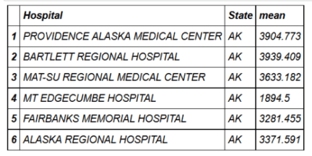
mygroup= group_by(hospital_spending,Hospital,State) from_dplyr = summarize(mygroup,mean=mean(Avg.Spending.Per.Episode..Hospital.)) from_data_table=hospital_spending_DT[,.(mean=mean(Avg.Spending.Per.Episode..Hospital.)), by=.(Hospital,State)] compare(from_dplyr,from_data_table, allowAll=TRUE)
TRUE sorted renamed rows dropped row names dropped attributes
シリアル接続
dplyrと
data.table両方
dplyr 、関数チェーンを構築できます。
dplyr 、
magrittrパッケージのパイプラインを
%>%使用できます。
%>%は、1つの関数の結果を最初の引数として次の引数に渡します。
data.tableでは、
%>%または
[チェーンの構築に使用されます。
from_dplyr=hospital_spending%>%group_by(Hospital,State)%>%summarize(mean=mean(Avg.Spending.Per.Episode..Hospital.)) from_data_table=hospital_spending_DT[,.(mean=mean(Avg.Spending.Per.Episode..Hospital.)), by=.(Hospital,State)] compare(from_dplyr,from_data_table, allowAll=TRUE)
TRUE sorted renamed rows dropped row names dropped attributes
hospital_spending%>%group_by(State)%>%summarize(mean=mean(Avg.Spending.Per.Episode..Hospital.))%>% arrange(desc(mean))%>%head(10)%>% mutate(State = factor(State,levels = State[order(mean,decreasing =TRUE)]))%>% ggplot(aes(x=State,y=mean))+geom_bar(stat='identity',color='darkred',fill='skyblue')+ xlab("")+ggtitle('Average Spending Per Episode by State')+ ylab('Average')+ coord_cartesian(ylim = c(3800, 4000))
 州ごとのケースあたりの平均費用
 hospital_spending_DT[,.(mean=mean(Avg.Spending.Per.Episode..Hospital.)), by=.(State)][order(-mean)][1:10]%>% mutate(State = factor(State,levels = State[order(mean,decreasing =TRUE)]))%>% ggplot(aes(x=State,y=mean))+geom_bar(stat='identity',color='darkred',fill='skyblue')+ xlab("")+ggtitle('Average Spending Per Episode by State')+ ylab('Average')+ coord_cartesian(ylim = c(3800, 4000))
州ごとのケースあたりの平均費用おわりに
data.tableおよび
dplyrを使用して、同じ操作を実行する方法を検討しました。 各パッケージには独自の利点があります。
この記事で使用されるコードは
GitHubで入手でき
ます 。