こんにちは、Habr！最近、機械学習とデータサイエンス全体がますます一般的になっています。新しいライブラリは常に登場しており、機械学習モデルのトレーニングに必要なコードはごくわずかです。そのような状況では、機械学習はそれ自体が目的ではなく、問題を解決するためのツールであることを忘れることができます。作業モデルを作成するだけでは不十分です。分析の結果を定性的に提示するか、作業製品を作成することも同様に重要です。

ユーザーが描いた数字で再訓練されたモデルを使用して、数字の手書き認識のためのプロジェクトを作成した方法についてお話したいと思います。 2つのモデルが使用されます。純粋なnumpyの単純なニューラルネットワーク（FNN）とTensorflowの畳み込みネットワーク（CNN）です。次のことを最初から行う方法を学習できます。

FlaskとBootstrapを使用して簡単なサイトを作成します。
Herokuプラットフォームに配置します。
Amazon s3クラウドを使用してデータの保存と読み込みを実装する
独自のデータセットを構築します。
機械学習モデル（FNNおよびCNN）をトレーニングします。
これらのモデルを再トレーニングできるようにします。
描かれた画像を認識できるサイトを作ります。

プロジェクトを完全に理解するには、画像認識でディープラーニングがどのように機能するかを理解し、Flaskの基本的な知識と、HTML、JS、CSSの少しの知識が必要です。

私について少し

モスクワ州立大学経済学部を卒業後、ERPシステムの実装と開発の分野でITコンサルティングに4年間従事しました。働くことは非常に面白かったです。長年にわたって多くの有用なことを学びましたが、やがてそれが私のものではないことを理解するようになりました。よく考えてから、活動分野を変えて機械学習の方向に切り替えることにしました（誇大広告ではなく、本当に興味を持ったからです）。これを行うには、終了して約6か月間働いて、プログラミング、機械学習などの必要なことを個別に勉強しました。その後、困難を伴いますが、それでもこの方向で作業が見つかりました。暇なときにスキルを開発し、活気づけようとしています。

アイデアの起源

数か月前、私はCourseraでYandexとMIPTの専門化を完了しました。彼女はSlackに自分のチームを持ち、4月にそこでスタンフォードのcs231nコースのためにグループを編成しました。これがどのように起こったかは別の話ですが、ポイントに近いです。コースの重要な部分は独立したプロジェクト（学生の成績の40％）であり、これにより行動の完全な自由が提供されます。真剣に何かをして、それについて記事を書くことの意味がわかりませんでしたが、それでも私の魂は私に尊厳をもってコースを終えるように頼みました。この頃、Tensorflowで数字と2つのグリッドを描画できるWebサイトに出会い、即座にそれを認識して結果を表示しました。同様のことを行うことにしましたが、データとモデルを使用しました。

本体

ここでは、プロジェクトを実装するために何をどのように行ったかについて説明します。説明は、行われたことを繰り返すことができるほど十分に詳細になりますが、基本的なことを簡単に説明するかスキップします。

プロジェクト計画

大きな何かに着手する前に、何かを計画する価値があります。その過程で、新しい詳細が明らかになり、計画を修正する必要がありますが、いくつかの最初のビジョンを修正する必要があります。

機械学習プロジェクトの基本的な問題の1つは、どのデータを使用し、どこで取得するかという問題です。 MNISTデータセットは、数字認識の問題で積極的に使用されているため、使用したくありませんでした。インターネットでは、MNISTでモデルがトレーニングされる同様のプロジェクトの例があります（たとえば、前述の）が、何か新しいことをしたかったのです。そして最後に、MNISTの数字の多くは現実からかけ離れているように思えました-データセットを見ると、現実には想像しにくい多くのオプションに出くわしました（その人が本当にひどい手書き文字を持っている場合を除く）。さらに、ブラウザでマウスを使用して数字を描くことは、ペンで数字を書くこととは多少異なります。その結果、私は自分のデータセットをまとめることにしました。
次の（または、同時に）ステップは、データを収集するためのWebサイトを作成することです。当時、私はFlaskの基本的な知識だけでなく、HTML、JS、CSSについても知っていました。したがって、Flaskにサイトを作成することにしました。Herokuがホスティングとして選択されました。小さなサイトをすばやく簡単にホストできるからです。
次に、モデル自体を作成する必要がありました。これにより、主な作業が行われます。 cs231nの後、画像認識用のニューラルネットワークアーキテクチャを作成するのに十分な経験があったため、この手順は最も簡単に思えました。以前は、いくつかのモデルを作成したかったのですが、後にFNNとCNNの2つに焦点を合わせることにしました。さらに、これらのモデルをトレーニングできるようにする必要がありました。このテーマについてはすでにいくつかのアイデアがありました。
モデルを準備した後、サイトを適切な外観にし、何らかの形で予測を表示し、答えの正しさを評価し、機能を少し説明し、その他多くの小さくてあまりないことを行う機会を与えます。計画の段階で、私はそれについて考えることに多くの時間を費やさず、単にリストを作成しました。

データ収集

プロジェクトに費やした時間のほぼ半分がデータ収集に費やされました。事実、私は何をしなければならないかについてほとんど知らなかったので、試行錯誤を繰り返す必要がありました。当然、複雑なのは図面自体ではなく、数字を描画してどこかに保存するサイトの作成です。これを行うには、Flaskをよりよく理解し、Javascriptを掘り下げ、Amazon S3クラウドを理解し、Herokuについて学ぶ必要がありました。私はプロジェクトの最初に持っていたのと同じレベルの知識を持って、それを繰り返すことができるように、これらすべてを十分詳細に説明します。

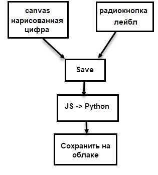
以前、私はこの図を描きました：

データ収集自体は数日、まあ、または数時間の純粋な時間を要しました。私は1000桁、それぞれ約100桁（正確ではない）を描画し、異なるスタイルで描画しようとしましたが、もちろん、可能なすべての手書きオプションをカバーすることはできませんでしたが、それは目標ではありませんでした。

サイトの最初のバージョンの作成（データ収集用）

サイトの最初のバージョンは次のようになりました。

最も基本的な機能しかありませんでした。

描画用のキャンバス。
ラベルを選択するためのラジオボタン。
画像を保存し、キャンバスをクリーニングするためのボタン。
保存が正常に書き込まれたフィールド。
Amazonクラウドに写真を保存します。

それで、これについてもっと詳しく説明しましょう。特にこの記事では、最小限の機能を備えたバージョンのサイトを作成しました。この例では、上記の方法を説明します。

注：サイトが長い間誰かによって開かれていない場合、サイトの起動には最大20〜30秒かかります。これはホスティングの無料バージョンのコストです。この状況は、サイトのフルバージョンに関連しています。

フラスコについて簡単に

Flaskは、Webサイトを作成するためのPythonフレームワークです。公式ウェブサイトには素晴らしい紹介があります。 Flaskを使用して情報を送受信するさまざまな方法があるため、このプロジェクトではAJAXを使用しました。 AJAXは、ブラウザとWebサーバー間でデータを「バックグラウンド」で交換する機能を提供します。これにより、データを転送するたびにページをリロードする必要がなくなります。

プロジェクト構造

プロジェクトで使用されるすべてのファイルは、2つの等しくないグループに分けることができます。アプリケーションがHerokuで動作するために必要な部分は小さく、残りはすべてサイトの作業に直接関与します。

HTMLとJS

HTMLファイルはテンプレートフォルダーに保存する必要があります。この段階では、テンプレートフォルダーがあれば十分です。ドキュメントヘッダーとbodyタグの最後には、jsファイルとcssファイルへのリンクがあります。これらのファイル自体は、「静的」フォルダーになければなりません。

HTMLファイル

<!doctype html> <html> <head> <meta charset="utf-8" /> <title>Handwritten digit recognition</title> <link rel="stylesheet" type="text/css" href="static/bootstrap.min.css"> <link rel="stylesheet" type="text/css" href="static/style.css"> </head> <body> <div class="container"> <div>   . <canvas id="the_stage" width="200" height="200">fsf</canvas> <div> <button type="button" class="btn btn-default butt" onclick="clearCanvas()"><strong>clear</strong></button> <button type="button" class="btn btn-default butt" id="save" onclick="saveImg()"><strong>save</strong></button> </div> <div> Please select one of the following <input type="radio" name="action" value="0" id="digit">0 <input type="radio" name="action" value="1" id="digit">1 <input type="radio" name="action" value="2" id="digit">2 <input type="radio" name="action" value="3" id="digit">3 <input type="radio" name="action" value="4" id="digit">4 <input type="radio" name="action" value="5" id="digit">5 <input type="radio" name="action" value="6" id="digit">6 <input type="radio" name="action" value="7" id="digit">7 <input type="radio" name="action" value="8" id="digit">8 <input type="radio" name="action" value="9" id="digit">9 </div> </div> <div class="col-md-6 column"> <h3>result:</h3> <h2 id="rec_result"></h2> </div> </div> <script src="static/jquery.min.js"></script> <script src="static/bootstrap.min.js"></script> <script src="static/draw.js"></script> </body></html>

キャンバスでの描画方法と描画の保存方法について詳しく説明します。
Canvasは2次元のHTML5描画要素です。画像はスクリプトを使用して描画することも、ユーザーがマウスを使用して（またはタッチスクリーンに触れて）描画することもできます。

Canvasは、HTMLで次のように定義されています。

 <canvas id="the_stage" width="200" height="200"> </canvas>

それ以前は、このHTML要素に慣れていなかったため、描画を可能にする最初の試みは失敗しました。しばらくして、実用的な例を見つけて借りました（リンクはdraw.jsファイルにあります）。

描画用コード

 var drawing = false; var context; var offset_left = 0; var offset_top = 0; function start_canvas () { var canvas = document.getElementById ("the_stage"); context = canvas.getContext ("2d"); canvas.onmousedown = function (event) {mousedown(event)}; canvas.onmousemove = function (event) {mousemove(event)}; canvas.onmouseup = function (event) {mouseup(event)}; for (var o = canvas; o ; o = o.offsetParent) { offset_left += (o.offsetLeft - o.scrollLeft); offset_top += (o.offsetTop - o.scrollTop); } draw(); } function getPosition(evt) { evt = (evt) ? evt : ((event) ? event : null); var left = 0; var top = 0; var canvas = document.getElementById("the_stage"); if (evt.pageX) { left = evt.pageX; top = evt.pageY; } else if (document.documentElement.scrollLeft) { left = evt.clientX + document.documentElement.scrollLeft; top = evt.clientY + document.documentElement.scrollTop; } else { left = evt.clientX + document.body.scrollLeft; top = evt.clientY + document.body.scrollTop; } left -= offset_left; top -= offset_top; return {x : left, y : top}; } function mousedown(event) { drawing = true; var location = getPosition(event); context.lineWidth = 8.0; context.strokeStyle="#000000"; context.beginPath(); context.moveTo(location.x,location.y); } function mousemove(event) { if (!drawing) return; var location = getPosition(event); context.lineTo(location.x,location.y); context.stroke(); } function mouseup(event) { if (!drawing) return; mousemove(event); context.closePath(); drawing = false; } . . . onload = start_canvas;

描画の仕組み

ページがロードされると、start_canvas関数が起動します。最初の2行は、特定のID（「ステージ」）を持つ要素としてキャンバスを見つけ、2次元画像として定義します。キャンバスに描画する場合、onmousedown、onmousemove、onmouseupの3つのイベントがあります。タッチについても同様のイベントがありますが、それについては後で詳しく説明します。

onmousedown-キャンバスをクリックすると発生します。この時点で、線の幅と色が設定され、描画の開始点も決定されます。つまり、カーソルの位置を決定することは簡単に聞こえますが、実際には完全に簡単ではありません。 getPosition（）関数は、ポイントを見つけるために使用されます-ページ上のカーソルの座標を見つけ、ページ上のキャンバスの相対位置を考慮し、ページがスクロールできることを考慮して、キャンバス上のポイントの座標を決定します。ポイントを見つけた後、 context.beginPath（）は描画パスを開始し、 context.moveTo（location.x、location.y）は、クリック時に決定されたポイントにこのパスを「移動」します。

onmousemove-左ボタンを押したままマウスの動きを追跡します。最初に、キーが押された（つまり、drawing = true）ことを確認しました。そうでない場合、描画は実行されません。 context.lineTo（）はマウスのパスに沿って線を作成し、 context.stroke（）はそれを直接描画します。
onmouseup-マウスの左ボタンが離されると発生します。 context.closePath（）は、線の描画を完了します。

インターフェースにはさらに4つの要素があります。

現在のステータスの「フィールド」。 JSはid（rec_result）でアクセスし、現在のステータスを表示します。ステータスは空であるか、画像が保存されていることを示すか、保存された画像の名前を示します。

  <div class="col-md-6 column"> <h3>result:</h3> <h2 id="rec_result"></h2> </div>

数字を選択するためのラジオボタン。データ収集段階では、描画された番号に何らかの方法でラベルを割り当てる必要があります。この10個のボタンが追加されたためです。ボタンは次のように設定されます。
```
 <input type="radio" name="action" value="0" id="digit">0 
```
ここで、0の代わりに対応する数字があります。 JSがアクティブなラジオボタンの値（ value ）を取得できるように、 名前が使用されます。
キャンバスをクリアするボタン-新しい番号を描画できるようにします。
```
 <button type="button" class="btn btn-default butt" onclick="clearCanvas()"><strong>clear</strong></button> 
```
このボタンをクリックすると、次のことが起こります。

 function draw() { context.fillStyle = '#ffffff'; context.fillRect(0, 0, 200, 200); } function clearCanvas() { context.clearRect (0, 0, 200, 200); draw(); document.getElementById("rec_result").innerHTML = ""; }

キャンバスの内容がクリアされ、白で塗りつぶされます。また、ステータスは空になります。

最後に、描かれた画像を保存するボタン。次のJavaScript関数を呼び出します。

 function saveImg() { document.getElementById("rec_result").innerHTML = "connecting..."; var canvas = document.getElementById("the_stage"); var dataURL = canvas.toDataURL('image/jpg'); var dig = document.querySelector('input[name="action"]:checked').value; $.ajax({ type: "POST", url: "/hook", data:{ imageBase64: dataURL, digit: dig } }).done(function(response) { console.log(response) document.getElementById("rec_result").innerHTML = response }); }

ボタンをクリックした直後に、ステータスフィールドに「接続中...」の値が表示されます。その後、画像はbase64エンコード方式を使用してテキスト文字列に変換されます。結果は次のとおりです： data:image/png;base64,%string% 、ファイルタイプ（image）、拡張子（png）、base64エンコーディング、および文字列自体を確認できます。ここで、コードの間違いに遅すぎることに気付きました。 canvas.toDataURL()引数として「image / jpeg」を使用する必要がありましたが、タイプミスを行った結果、画像は実際にはpngでした。

次に、アクティブラジオボタンの値（名前= 'action'でchecked ）を取得し、 dig変数に保存します。

最後に、AJAX要求はエンコードされた画像とラベルをpythonに送信し、応答を受け取ります。この設計を機能させるために多くの時間を費やしました。各行で何が起こるかを説明しようとします。

まず、リクエストのタイプが示されます-この場合、「POST」、つまり、JSからのデータがpythonスクリプトに転送されます。

「/フック」は、データが転送される場所です。 Flaskを使用しているため、必要なデコレーターでURLとして「/ hook」を指定できます。これは、POST要求がこのURLに送信されるときに使用されるのはこのデコレーターの関数であることを意味します。詳細については、以下のフラスコのセクションを参照してください。

dataは、リクエストで送信されるデータです。データの送信には多くのオプションがあります。この場合、値と、この値を取得できる名前を設定します。
最後に、 done()はリクエストが成功したときに起こることです。私のAJAXリクエストは特定の回答（より正確には、保存された画像の名前を含むテキスト）を返します。この回答は、最初にコンソールに表示され（デバッグ用）、次にステータスフィールドに表示されます。

気を散らすために、プロジェクトの作業の開始時に生じた小さな問題についてお話したいと思います。何らかの理由で、この画像処理の基本的なサイトの読み込みには約1分かかりました。数行だけを残して最小化しようとしましたが、何も助けにはなりませんでした。その結果、コンソールのおかげで、ブレーキの原因を特定することができました-アンチウイルス。

Kasperskyが自分のサイトにスクリプトを挿入したため、ダウンロードに時間がかかりました。オプションを無効にした後、サイトはすぐにロードし始めました。

フラスコと画像保存

それでは、AJAXリクエストからのデータがどのようにpythonに送られ、画像がどのように保存されるかを見ていきましょう。

Flaskの操作に関するガイドや記事は多数あります。そのため、基本的なことを簡単に説明し、コードが機能しない行に特に注意を払います。もちろん、サイトの基本である残りのコードについても説明します。

main.py

 __author__ = 'Artgor' from functions import Model from flask import Flask, render_template, request from flask_cors import CORS, cross_origin import base64 import os app = Flask(__name__) model = Model() CORS(app, headers=['Content-Type']) @app.route("/", methods=["POST", "GET", 'OPTIONS']) def index_page(): return render_template('index.html') @app.route('/hook', methods = ["GET", "POST", 'OPTIONS']) def get_image(): if request.method == 'POST': image_b64 = request.values['imageBase64'] drawn_digit = request.values['digit'] image_encoded = image_b64.split(',')[1] image = base64.decodebytes(image_encoded.encode('utf-8')) save = model.save_image(drawn_digit, image) print('Done') return save if __name__ == '__main__': port = int(os.environ.get("PORT", 5000)) app.run(host='0.0.0.0', port=port, debug=False)

functions.py

 __author__ = 'Artgor' from codecs import open import os import uuid import boto3 from boto.s3.key import Key from boto.s3.connection import S3Connection class Model(object): def __init__(self): self.nothing = 0 def save_image(self, drawn_digit, image): filename = 'digit' + str(drawn_digit) + '__' + str(uuid.uuid1()) + '.jpg' with open('tmp/' + filename, 'wb') as f: f.write(image) print('Image written') REGION_HOST = 's3-external-1.amazonaws.com' conn = S3Connection(os.environ['AWS_ACCESS_KEY_ID'], os.environ['AWS_SECRET_ACCESS_KEY'], host=REGION_HOST) bucket = conn.get_bucket('testddr') k = Key(bucket) fn = 'tmp/' + filename k.key = filename k.set_contents_from_filename(fn) print('Done') return ('Image saved successfully with the name {0}'.format(filename))

コードの仕組み

最初のステップは、デフォルト値app = Flask(__name__) Flaskクラスのインスタンスを作成することです。これがアプリケーションの基礎になります。

次に、2番目のスクリプトを使用するクラスのインスタンスを作成します。関数が1つしかない場合、クラスを使用せずに実行することも、1つのスクリプトですべてのコードを保持することもできます。しかし、メソッドの数が増えることはわかっていたので、すぐにこのオプションを使用することにしました。

CORS（クロスオリジンリソース共有）は、Webページに別のドメインのリソースへのアクセスを提供する技術です。このアプリケーションでは、これを使用してAmazonクラウドに画像を保存します。私は長い間この設定を有効にする方法を探していましたが、それを簡単にする方法を探していました。その結果、 CORS(app, headers=['Content-Type']) 1行で実装しました。

次に、 route()デコレータが使用されます-どの関数がどのURLに対して実行されるかを決定します。メインスクリプトには、関数を持つ2つのデコレータがあります。最初のページはメインページに使用され（アドレスは"/" ）、 "index.html"を表示します。 2番目のデコレーターにはアドレス「 "/ hook"」があります。これは、JSからのデータがそこに転送されることを意味します（同じアドレスがそこに指定されたことを思い出します）。

どちらのデコレーターにも、メソッドパラメーターの値として「POST」、「GET」、「OPTIONS」のリストがあることに注意してください。 POSTとGETはデータの送受信に使用され（両方とも念のため）、CORSなどのパラメーターを渡すにはOPTIONSが必要です。理論的には、Flaskバージョン0.6からOPTIONSをデフォルトで使用する必要がありますが、明示的な指示がないと、コードを動作させることができませんでした。

次に、画像を取得する機能について説明します。 JSからPythonへの「リクエスト」があります。これは、フォームからのデータ、AJAXから取得したデータなどです。私の場合、これはキーと値がJSで指定された辞書です。画像のラベルの抽出は簡単で、キーごとに辞書の値を取得する必要がありますが、画像を含む文字列を処理する必要があります-画像自体に関連する部分を取得し（説明を破棄）、デコードします。

その後、2番目のスクリプトの関数が呼び出され、画像が保存されます。保存された画像の名前を含む文字列を返します。その後、JSに戻り、ブラウザページに表示されます。

コードの最後の部分は、アプリケーションがherokuで動作するために必要です（ドキュメントから取得）。 Herokuにアプリケーションを配置する方法については、対応するセクションで詳しく説明します。

最後に、画像がどのように保存されるかを見てみましょう。現在、画像は変数に保存されていますが、画像をAmazonクラウドに保存するにはファイルが必要なので、画像を保存する必要があります。画像の名前には、ラベルと、uuidを使用して生成された一意のIDが含まれます。その後、画像は一時的なtmpフォルダーに保存され、クラウドにアップロードされます。 tmpフォルダー内のファイルは一時的なものであるとすぐに言っておく必要があります。herokuはセッション中に新しい/変更されたファイルを保存し、終了時にファイルを削除するか、変更をロールバックします。これにより、フォルダーをクリアする必要性について考える必要がなくなり、一般的に便利ですが、クラウドを使用する必要があるのはまさにこのためです。

これで、Amazonクラウドの仕組みと、それを使って何ができるかについて話すことができます。

Amazon S3の統合

Pythonには、botoとboto3の2つのAmazonクラウドライブラリがあります。 2番目の方法はより新しく、より適切にサポートされていますが、これまでのところ、最初の方法を使用した方が便利な場合があります。

Amazonでバケットを構築および構成する

アカウントを登録しても問題はないと思います。ライブラリを使用してアクセスするためのキー（アクセスキーIDとシークレットアクセスキー）を生成することを忘れないことが重要です。クラウド自体で、ファイルを保存するバケットを作成できます。ロシア語では、バケツはバケツであり、私には奇妙に聞こえるので、元の名前を使用することを好みます。
そして今、ニュアンスはなくなっています。

作成するときは、名前を指定する必要があり、ここでは注意する必要があります。最初は、ハイフンでつながれた名前を使用しましたが、クラウドに接続できませんでした。いくつかの個々のキャラクターがこの問題を引き起こすことが判明しました。回避策はありますが、すべての人に役立つわけではありません。その結果、アンダースコア（digit_draw_recognize）で名前の変形を使用し始めましたが、問題はありませんでした。
次に、地域を指定する必要があります。ほとんどすべてを選択できますが、このプレートにガイドされる必要があります。
まず、選択したリージョンにエンドポイントが必要です。次に、便利なものを使用できるように、2および4バージョンの署名をサポートするリージョンを使用する方が簡単です。米国東部（バージニア北部）を選びました。

バケット作成時の他のパラメーターは変更できません。
もう1つの重要なポイントは、CORSの構成です。

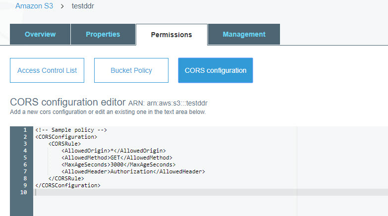
次のコードを構成に入力する必要があります。

 <CORSConfiguration> <CORSRule> <AllowedOrigin>*</AllowedOrigin> <AllowedMethod>GET</AllowedMethod> <MaxAgeSeconds>3000</MaxAgeSeconds> <AllowedHeader>Authorization</AllowedHeader> </CORSRule> </CORSConfiguration>

この設定の詳細についてはこちらをご覧ください。ソフト/タフなパラメーターを設定できます。最初は、（GETだけでなく）より多くのメソッドを指定する必要があると思いましたが、すべてそのように動作しました。

さて、実際にコードについて話す。ここでは、ファイルをAmazonに保存する方法のみに焦点を当てます。クラウドからのデータの受信については、少し後で説明します。

 REGION_HOST = 's3-external-1.amazonaws.com' conn = S3Connection(os.environ['AWS_ACCESS_KEY_ID'], os.environ['AWS_SECRET_ACCESS_KEY'], host=REGION_HOST) bucket = conn.get_bucket('testddr') k = Key(bucket) fn = 'tmp/' + filename k.key = filename k.set_contents_from_filename(fn)

最初のステップは、クラウド接続を作成することです。これを行うには、アクセスキーID、シークレットアクセスキー、およびリージョンホストを指定します。キーはすでに生成されていますが、明示的に指定することは危険です。これは、コードをローカルでテストするときにのみ実行できます。公然と指定されたキーを使用してgithubコードに数回コミットしました-それらは数分間盗まれました。私の間違いを繰り返さないでください。 Herokuには、キーを保存し、名前でアクセスする機能があります。詳細については、以下をご覧ください。リージョンホストは、リージョンラベルのエンドポイント値です。

その後、バケットに接続する必要があります-ここでは、名前を直接指定することは完全に受け入れられます。

Key 、バスケット内のオブジェクトを操作するために使用されます。オブジェクトを保存するには、ファイル名（k.key）を指定し、保存するファイルへのパスでk.set_contents_from_filename()を呼び出す必要があります。

ヘロク

Herokuでサイトをホストする方法について話します。 Herokuは、Webアプリケーションを迅速かつ便利に展開できる多言語クラウドプラットフォームです。 Postgresと多くの興味深いものを使用することが可能です。一般的に、Herokuリソースを使用して画像を保存できますが、異なる種類のデータを保存する必要があるため、別のクラウドを使用する方が簡単でした。

Herokuにはいくつかの価格プランがありますが、私のアプリケーション（この小さなプランではなく、本格的なプランを含む）には、無料のプランで十分です。唯一のマイナス点は、30分間のアクティビティの後、アプリケーションが「スリープ」状態になり、次に起動するときに「ウェイクアップ」に30秒を費やすことができることです。

ネットワーク上のHerokuにアプリケーションをデプロイするためのガイドは多数あります（公式リンクへのリンクはこちら）が、それらのほとんどはコンソールを使用しており、インターフェイスを使用することを好みます。さらに、私にとってはずっとシンプルで便利なようです。

Herokuでのアプリホスティング

だからポイントに。アプリケーションを準備するには、いくつかのファイルを作成する必要があります。

バージョン管理システム.gitが必要です。通常、githubリポジトリを作成すると自動的に作成されますが、実際に作成されていることを確認する必要があります。
runtime.txtこのファイルでは、プログラミング言語の必要なバージョンを示す必要があります。私の場合はpython-3.6.1。
Procfileは、拡張子のないファイルです。 herokuで実行するコマンドを示します。これにより、開始するwebプロセスのタイプ（私のスクリプト）とアドレスが決まります。

 web: python main.py runserver 0.0.0.0:5000

requirements.txt -Herokuにインストールされるライブラリのリスト。必要なバージョンを示すことをお勧めします。
最後の-少なくとも1つのファイルが「tmp」フォルダーにある必要があります。そうでない場合、アプリケーション操作中にこのフォルダーにファイルを保存する際に問題が発生する可能性があります。

これで、アプリケーションの作成プロセスを開始できます。この時点で、herokuのアカウントと準備済みのgithubリポジトリが必要です。

アプリケーションのリストを含むページから、新しいものが作成されます。

名前と国を示します。

[デプロイ]タブで、Githubへの接続を選択します。

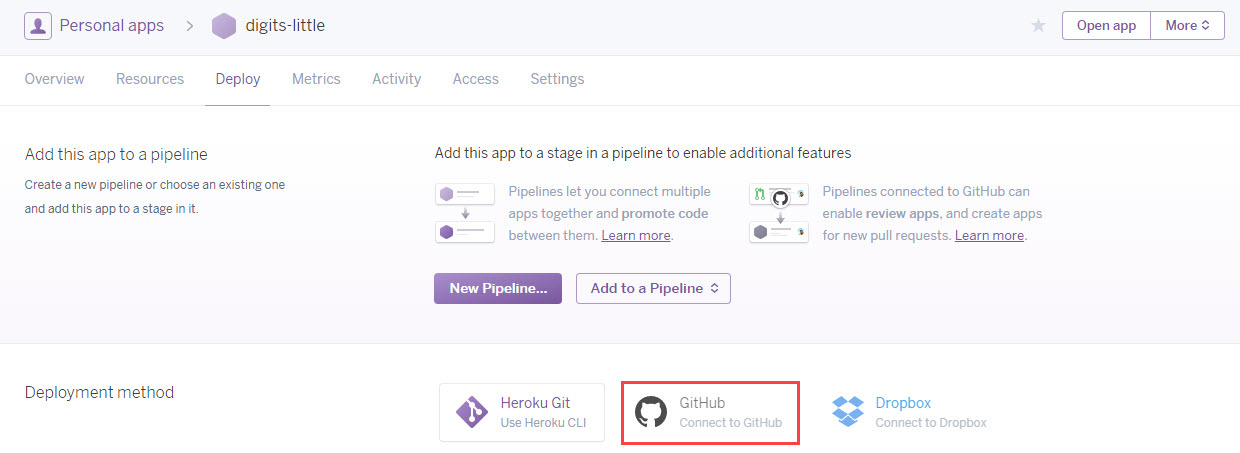
リポジトリを接続して選択します。

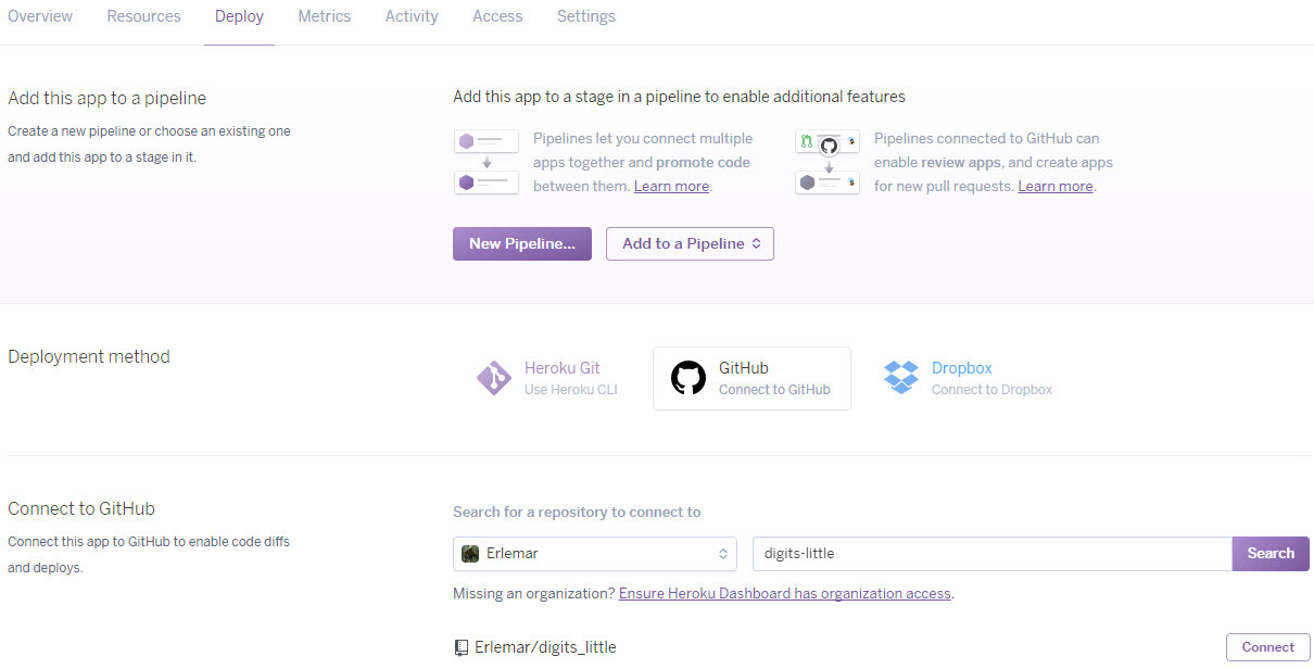
リポジトリが更新されるたびにHerokuでアプリケーションの自動更新を有効にすることは理にかなっています。そして、展開を開始できます。

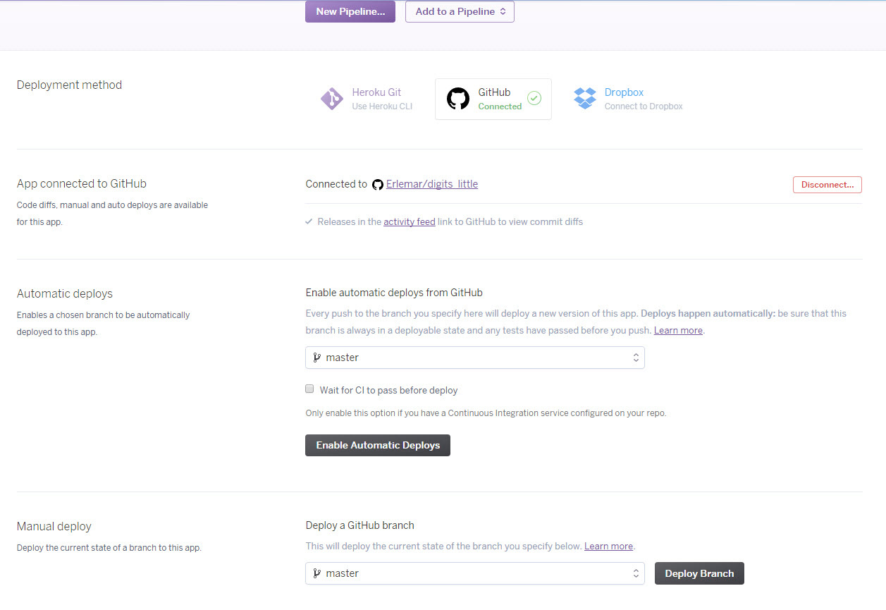
ログを見て、すべてがうまくいったことを願っています。

しかし、すべてがまだ準備ができているわけではありません。設定タブでアプリケーションを最初に起動する前に、変数-Amazonクラウドのキーを設定する必要があります。

これで、アプリケーションを実行して操作できるようになりました。これで、データ収集サイトの説明は完了です。さらに、データ処理とプロジェクトの次の段階に焦点を当てます。

モデルの画像処理

描画された画像を元の形式で画像として保存します。これにより、常にそれらを表示して、さまざまな処理オプションを試すことができます。

以下に例を示します。

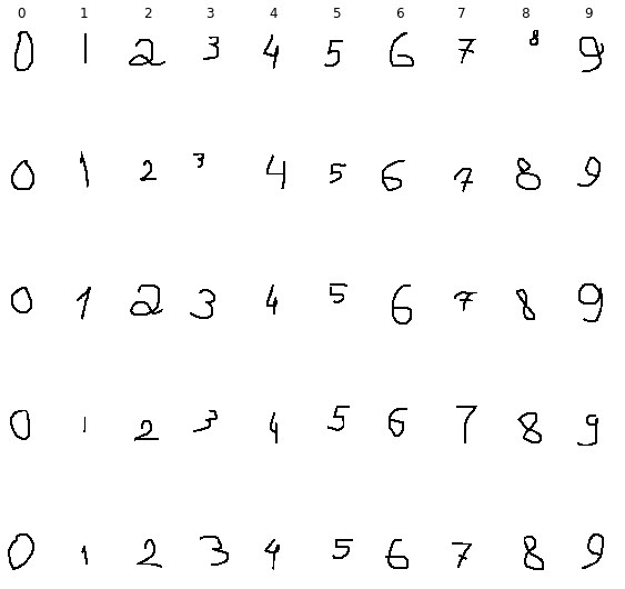
私のプロジェクトの画像処理のアイデアは次のとおりです（mnistに似ています）：描かれた数字は、20x20の正方形に収まるようにスケーリングされ、比率が保たれ、28x28の大きさの白い正方形の中央に配置されます。これを行うには、次の手順が必要です。

画像の境界線を見つける（境界線は長方形の形をしています）;
境界矩形の高さと幅を見つけます。
大きい側を20に等しくし、小さい側をスケーリングして比率を維持します。
28x28の正方形にスケーリングされた図形を描画するための開始点を見つけて描画します。
データを操作して正規化できるように、np.arrayに変換します。

画像処理

 #    img = Image.open('tmp/' + filename) #   bbox = Image.eval(img, lambda px: 255-px).getbbox() if bbox == None: return None #    widthlen = bbox[2] - bbox[0] heightlen = bbox[3] - bbox[1] #  if heightlen > widthlen: widthlen = int(20.0 * widthlen / heightlen) heightlen = 20 else: heightlen = int(20.0 * widthlen / heightlen) widthlen = 20 #    hstart = int((28 - heightlen) / 2) wstart = int((28 - widthlen) / 2) #   img_temp = img.crop(bbox).resize((widthlen, heightlen), Image.NEAREST) #       new_img = Image.new('L', (28,28), 255) new_img.paste(img_temp, (wstart, hstart)) #   np.array   imgdata = list(new_img.getdata()) img_array = np.array([(255.0 - x) / 255.0 for x in imgdata])

画像増強

明らかに、1000個の画像はニューラルネットワークのトレーニングには不十分であり、それらの一部はモデルの検証に使用する必要があります。この問題の解決策は、データの増強です。データセットのサイズを増やすのに役立つ追加の画像を作成します。 , , . .

, . 2020 . 4 — 4 .

. , — 30 ; 5 , 12 . , 12 6.

 #    image = Image.open('tmp/' + filename) #        ims_add = [] labs_add = [] # ,       angles = np.arange(-30, 30, 5) #   bbox = Image.eval(image, lambda px: 255-px).getbbox() #    widthlen = bbox[2] - bbox[0] heightlen = bbox[3] - bbox[1] #  if heightlen > widthlen: widthlen = int(20.0 * widthlen/heightlen) heightlen = 20 else: heightlen = int(20.0 * widthlen/heightlen) widthlen = 20 #    hstart = int((28 - heightlen) / 2) wstart = int((28 - widthlen) / 2) # 4   for i in [min(widthlen, heightlen), max(widthlen, heightlen)]: for j in [min(widthlen, heightlen), max(widthlen, heightlen)]: #   resized_img = image.crop(bbox).resize((i, j), Image.NEAREST) #       resized_image = Image.new('L', (28,28), 255) resized_image.paste(resized_img, (wstart, hstart)) #   6   12. angles_ = random.sample(set(angles), 6) for angle in angles_: #   transformed_image = transform.rotate(np.array(resized_image), angle, cval=255, preserve_range=True).astype(np.uint8) labs_add.append(int(label)) #      img_temp = Image.fromarray(np.uint8(transformed_image)) #   np.array   imgdata = list(img_temp.getdata()) normalized_img = [(255.0 - x) / 255.0 for x in imgdata] ims_add.append(normalized_img)

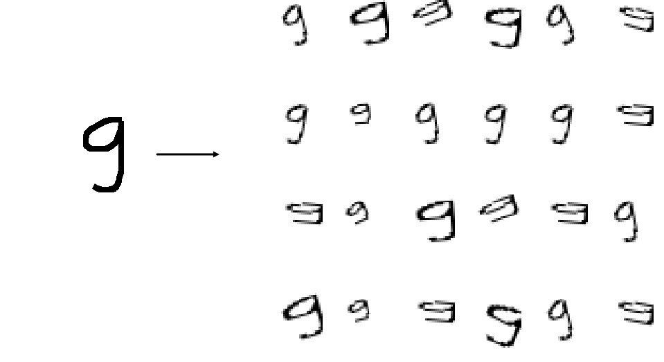
800 * 24 = 19200 200 . .

FNN

feed forward neural net. , cs231n, .

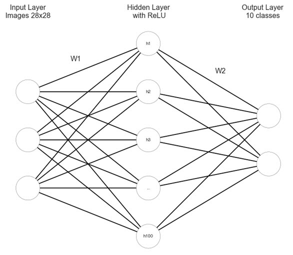
 import matplotlib.pyplot as plt #https://gist.github.com/anbrjohn/7116fa0b59248375cd0c0371d6107a59 def draw_neural_net(ax, left, right, bottom, top, layer_sizes, layer_text=None): ''' :parameters: - ax : matplotlib.axes.AxesSubplot The axes on which to plot the cartoon (get eg by plt.gca()) - left : float The center of the leftmost node(s) will be placed here - right : float The center of the rightmost node(s) will be placed here - bottom : float The center of the bottommost node(s) will be placed here - top : float The center of the topmost node(s) will be placed here - layer_sizes : list of int List of layer sizes, including input and output dimensionality - layer_text : list of str List of node annotations in top-down left-right order ''' n_layers = len(layer_sizes) v_spacing = (top - bottom)/float(max(layer_sizes)) h_spacing = (right - left)/float(len(layer_sizes) - 1) ax.axis('off') # Nodes for n, layer_size in enumerate(layer_sizes): layer_top = v_spacing*(layer_size - 1)/2. + (top + bottom)/2. for m in range(layer_size): x = n*h_spacing + left y = layer_top - m*v_spacing circle = plt.Circle((x,y), v_spacing/4., color='w', ec='k', zorder=4) ax.add_artist(circle) # Node annotations if layer_text: text = layer_text.pop(0) plt.annotate(text, xy=(x, y), zorder=5, ha='center', va='center') # Edges for n, (layer_size_a, layer_size_b) in enumerate(zip(layer_sizes[:-1], layer_sizes[1:])): layer_top_a = v_spacing*(layer_size_a - 1)/2. + (top + bottom)/2. layer_top_b = v_spacing*(layer_size_b - 1)/2. + (top + bottom)/2. for m in range(layer_size_a): for o in range(layer_size_b): line = plt.Line2D([n*h_spacing + left, (n + 1)*h_spacing + left], [layer_top_a - m*v_spacing, layer_top_b - o*v_spacing], c='k') ax.add_artist(line) node_text = ['','','','h1','h2','h3','...', 'h100'] fig = plt.figure(figsize=(8, 8)) ax = fig.gca() draw_neural_net(ax, .1, .9, .1, .9, [3, 5, 2], node_text) plt.text(0.1, 0.95, "Input Layer\nImages 28x28", ha='center', va='top', fontsize=16) plt.text(0.26, 0.78, "W1", ha='center', va='top', fontsize=16) plt.text(0.5, 0.95, "Hidden Layer\n with ReLU", ha='center', va='top', fontsize=16) plt.text(0.74, 0.74, "W2", ha='center', va='top', fontsize=16) plt.text(0.88, 0.95, "Output Layer\n10 classes", ha='center', va='top', fontsize=16) plt.show()

FNN

 import numpy as np class TwoLayerNet(object): """ A two-layer fully-connected neural network. The net has an input dimension of N, a hidden layer dimension of H, and performs classification over C classes. We train the network with a softmax loss function and L2 regularization on the weight matrices. The network uses a ReLU nonlinearity after the first fully connected layer. In other words, the network has the following architecture: input - fully connected layer - ReLU - fully connected layer - softmax The outputs of the second fully-connected layer are the scores for each class. """ def __init__(self, input_size, hidden_size, output_size, std): """ Initialize the model. Weights are initialized following Xavier intialization and biases are initialized to zero. Weights and biases are stored in the variable self.params, which is a dictionary with the following keys: W1: First layer weights; has shape (D, H) b1: First layer biases; has shape (H,) W2: Second layer weights; has shape (H, C) b2: Second layer biases; has shape (C,) Inputs: - input_size: The dimension D of the input data. - hidden_size: The number of neurons H in the hidden layer. - output_size: The number of classes C. """ self.params = {} self.params['W1'] = (((2 / input_size) ** 0.5) * np.random.randn(input_size, hidden_size)) self.params['b1'] = np.zeros(hidden_size) self.params['W2'] = (((2 / hidden_size) ** 0.5) * np.random.randn(hidden_size, output_size)) self.params['b2'] = np.zeros(output_size) def loss(self, X, y=None, reg=0.0): """ Compute the loss and gradients for a two layer fully connected neural network. Inputs: - X: Input data of shape (N, D). X[i] is a training sample. - y: Vector of training labels. y[i] is the label for X[i], and each y[i] is an integer in the range 0 <= y[i] < C. - reg: Regularization strength. Returns: - loss: Loss (data loss and regularization loss) for this batch of training samples. - grads: Dictionary mapping parameter names to gradients of those parameters with respect to the loss function; has the same keys as self.params. """ # Unpack variables from the params dictionary W1, b1 = self.params['W1'], self.params['b1'] W2, b2 = self.params['W2'], self.params['b2'] N, D = X.shape # Compute the forward pass l1 = X.dot(W1) + b1 l1[l1 < 0] = 0 l2 = l1.dot(W2) + b2 exp_scores = np.exp(l2) probs = exp_scores / np.sum(exp_scores, axis=1, keepdims=True) scores = l2 # Compute the loss W1_r = 0.5 * reg * np.sum(W1 * W1) W2_r = 0.5 * reg * np.sum(W2 * W2) loss = -np.sum(np.log(probs[range(y.shape[0]), y]))/N + W1_r + W2_r # Backward pass: compute gradients grads = {} probs[range(X.shape[0]),y] -= 1 dW2 = np.dot(l1.T, probs) dW2 /= X.shape[0] dW2 += reg * W2 grads['W2'] = dW2 grads['b2'] = np.sum(probs, axis=0, keepdims=True) / X.shape[0] delta = probs.dot(W2.T) delta = delta * (l1 > 0) grads['W1'] = np.dot(XT, delta)/ X.shape[0] + reg * W1 grads['b1'] = np.sum(delta, axis=0, keepdims=True) / X.shape[0] return loss, grads def train(self, X, y, X_val, y_val, learning_rate=1e-3, learning_rate_decay=0.95, reg=5e-6, num_iters=100, batch_size=24, verbose=False): """ Train this neural network using stochastic gradient descent. Inputs: - X: A numpy array of shape (N, D) giving training data. - y: A numpy array f shape (N,) giving training labels; y[i] = c means that [i] has label c, where 0 <= c < C. - X_val: A numpy array of shape (N_val, D); validation data. - y_val: A numpy array of shape (N_val,); validation labels. - learning_rate: Scalar giving learning rate for optimization. - learning_rate_decay: Scalar giving factor used to decay the learning rate each epoch. - reg: Scalar giving regularization strength. - num_iters: Number of steps to take when optimizing. - batch_size: Number of training examples to use per step. - verbose: boolean; if true print progress during optimization. """ num_train = X.shape[0] iterations_per_epoch = max(num_train / batch_size, 1) # Use SGD to optimize the parameters in self.model loss_history = [] train_acc_history = [] val_acc_history = [] # Training cycle for it in range(num_iters): # Mini-batch selection indexes = np.random.choice(X.shape[0], batch_size, replace=True) X_batch = X[indexes] y_batch = y[indexes] # Compute loss and gradients using the current minibatch loss, grads = self.loss(X_batch, y=y_batch, reg=reg) loss_history.append(loss) # Update weights self.params['W1'] -= learning_rate * grads['W1'] self.params['b1'] -= learning_rate * grads['b1'][0] self.params['W2'] -= learning_rate * grads['W2'] self.params['b2'] -= learning_rate * grads['b2'][0] if verbose and it % 100 == 0: print('iteration %d / %d: loss %f' % (it, num_iters, loss)) # Every epoch, check accuracy and decay learning rate. if it % iterations_per_epoch == 0: # Check accuracy train_acc = (self.predict(X_batch)==y_batch).mean() val_acc = (self.predict(X_val) == y_val).mean() train_acc_history.append(train_acc) val_acc_history.append(val_acc) # Decay learning rate learning_rate *= learning_rate_decay return { 'loss_history': loss_history, 'train_acc_history': train_acc_history, 'val_acc_history': val_acc_history, } def predict(self, X): """ Use the trained weights of this two-layer network to predict labels for points. For each data point we predict scores for each of the C classes, and assign each data point to the class with the highest score. Inputs: - X: A numpy array of shape (N, D) giving N D-dimensional data points to classify. Returns: - y_pred: A numpy array of shape (N,) giving predicted labels for each of elements of X. For all i, y_pred[i] = c means that X[i] is predicted to have class c, where 0 <= c < C. """ l1 = X.dot(self.params['W1']) + self.params['b1'] l1[l1 < 0] = 0 l2 = l1.dot(self.params['W2']) + self.params['b2'] exp_scores = np.exp(l2) probs = exp_scores / np.sum(exp_scores, axis=1, keepdims=True) y_pred = np.argmax(probs, axis=1) return y_pred def predict_single(self, X): """ Use the trained weights of this two-layer network to predict label for data point. We predict scores for each of the C classes, and assign the data point to the class with the highest score. Inputs: - X: A numpy array of shape (N, D) giving N D-dimensional data points to classify. Returns: - y_pred: A numpy array of shape (1,) giving predicted labels for X. """ l1 = X.dot(self.params['W1']) + self.params['b1'] l1[l1 < 0] = 0 l2 = l1.dot(self.params['W2']) + self.params['b2'] exp_scores = np.exp(l2) y_pred = np.argmax(exp_scores) return y_pred

FNN

cs231n :

— , , , .

, N 784, N — (19200 ). , , :

f (\sum_{i}^{n} x_{i} w_{i} + b)

$f(\sum_{i}^{n} x_{i}w_{i} + b)$

ReLU (Rectified Linear Unit),

l 1 = m a x (0, \sum_{i}^{n} x_{i} w_{i} + b)

$l1 = max(0, \sum_{i}^{n} x_{i}w_{i} + b)$

. ReLU , , sigmoid tahn; , ( ), learning rate . 784 100, N 100. :

l 2 = l 1 w^{h} + b

$l2 = l1w^{h} + b$

softmax, :

o u t = \frac{e^{f_{y_{i}}}}{\sum_{j} e^{f_{j}}}

$out = \frac{e^{f_{y_i}}}{ \sum_j e^{f_j} }$

, softmax — . , , . , 100 10, 10 , . Cross-entropy loss softmax :

L_{i} = - \log (\frac{e^{f_{y_{i}}}}{\sum_{j} e^{f_{j}}})

$L_i = -\log\left(\frac{e^{f_{y_i}}}{ \sum_j e^{f_j} }\right)$

(Xavier). 2 / . ;
loss L2 ;
train -. . , learning rate decay;
predict_single , predict — ;

 input_size = 28 * 28 hidden_size = 100 num_classes = 10 net = tln(input_size, hidden_size, num_classes)

;
-, ;
learning rate decay, learning rate ;
;
verbose / ;

 stats = net.train(X_train_, y_train_, X_val, y_val, num_iters=19200, batch_size=24, learning_rate=0.1, learning_rate_decay=0.95, reg=0.001, verbose=True)

, loss , :

 plt.subplot(2, 1, 1) plt.plot(stats['loss_history']) plt.title('Loss history') plt.xlabel('Iteration') plt.ylabel('Loss') plt.subplot(2, 1, 2) plt.plot(stats['train_acc_history'], label='train') plt.plot(stats['val_acc_history'], label='val') plt.title('Classification accuracy history') plt.xlabel('Epoch') plt.ylabel('Clasification accuracy') plt.legend() plt.show()

— . , , — , . . , , . , , , .

, . . learning rate, regularization, , -; , . .

 from itertools import product best_net = None results = {} best_val = -1 learning_rates = [0.001, 0.1, 0.01, 0.5] regularization_strengths = [0.001, 0.1, 0.01] hidden_size = [5, 10, 20] epochs = [1000, 1500, 2000] batch_sizes = [24, 12] best_params = 0 best_params = 0 for v in product(learning_rates, regularization_strengths, hidden_size, epochs, batch_sizes): print('learning rate: {0}, regularization strength: {1}, hidden size: {2}, \ iterations: {3}, batch_size: {4}.'.format(v[0], v[1], v[2], v[3], v[4])) net = TwoLayerNet(input_size, v[2], num_classes) stats = net.train(X_train_, y_train, X_val_, y_val, num_iters=v[3], batch_size=v[4], learning_rate=v[0], learning_rate_decay=0.95, reg=v[1], verbose=False) y_train_pred = net.predict(X_train_) train_acc = np.mean(y_train == y_train_pred) val_acc = (net.predict(X_val_) == y_val).mean() print('Validation accuracy: ', val_acc) results[(v[0], v[1], v[2], v[3], v[4])] = val_acc if val_acc > best_val: best_val = val_acc best_net = net best_params = (v[0], v[1], v[2], v[3], v[4])

, , , - . , , learning rate . . - , : , 1 . 1 24 , - . 24.

MNIST, MNIST.

MNIST

 def read(path = "."): fname_img = os.path.join(path, 't10k-images.idx3-ubyte') fname_lbl = os.path.join(path, 't10k-labels.idx1-ubyte') with open(fname_lbl, 'rb') as flbl: magic, num = struct.unpack(">II", flbl.read(8)) lbl = np.fromfile(flbl, dtype=np.int8) with open(fname_img, 'rb') as fimg: magic, num, rows, cols = struct.unpack(">IIII", fimg.read(16)) img = np.fromfile(fimg, dtype=np.uint8).reshape(len(lbl), rows, cols) get_img = lambda idx: (lbl[idx], img[idx]) for i in range(len(lbl)): yield get_img(i) test = list(read(path="/MNIST_data")) mnist_labels = np.array([i[0] for i in test]).astype(int) mnist_picts = np.array([i[1] for i in test]).reshape(10000, 784) / 255 y_mnist = np.array(mnist_labels).astype(int)

, ~10 , .

, , MNIST . , , MNIST . CNN Tensorflow MNIST . MNIST 99%+ ( ), : 78.5% 63.35% . , MNIST , MNIST.

, :

;
/;
: , , rmsprop;

. , .

: net.param , — , — . numpy : np.save('tmp/updated_weights.npy', net.params) . np.load('models/original_weights.npy')[()] ( [()] , ).

.

FNN

. :

, . ;
, ;
(1 , 24);
(learning rate ) ;
predict-single 3 . , ;

FNN

 import numpy as np class FNN(object): """ A two-layer fully-connected neural network. The net has an input dimension of N, a hidden layer dimension of H, and performs classification over C classes. We train the network with a softmax loss function and L2 regularization on the weight matrices. The network uses a ReLU nonlinearity after the first fully connected layer. In other words, the network has the following architecture: input - fully connected layer - ReLU - fully connected layer - softmax The outputs of the second fully-connected layer are the scores for each class. """ def __init__(self, weights,input_size=28*28,hidden_size=100,output_size=10): """ Initialize the model. Weights are initialized following Xavier intialization and biases are initialized to zero. Weights and biases are stored in the variable self.params, which is a dictionary with the following keys: W1: First layer weights; has shape (D, H) b1: First layer biases; has shape (H,) W2: Second layer weights; has shape (H, C) b2: Second layer biases; has shape (C,) Inputs: - input_size: The dimension D of the input data. - hidden_size: The number of neurons H in the hidden layer. - output_size: The number of classes C. """ self.params = {} self.params['W1'] = weights['W1'] self.params['b1'] = weights['b1'] self.params['W2'] = weights['W2'] self.params['b2'] = weights['b2'] def loss(self, X, y, reg=0.0): """ Compute the loss and gradients for a two layer fully connected neural network. Inputs: - X: Input data of shape (N, D). X[i] is a training sample. - y: Vector of training labels. y[i] is the label for X[i], and each y[i] is an integer in the range 0 <= y[i] < C. - reg: Regularization strength. Returns: - loss: Loss (data loss and regularization loss) for this batch of training samples. - grads: Dictionary mapping parameter names to gradients of those parameters with respect to the loss function; has the same keys as self.params. """ # Unpack variables from the params dictionary W1, b1 = self.params['W1'], self.params['b1'] W2, b2 = self.params['W2'], self.params['b2'] N, D = X.shape # Compute the forward pass l1 = X.dot(W1) + b1 l1[l1 < 0] = 0 l2 = l1.dot(W2) + b2 exp_scores = np.exp(l2) probs = exp_scores / np.sum(exp_scores, axis=1, keepdims=True) # Backward pass: compute gradients grads = {} probs[range(X.shape[0]), y] -= 1 dW2 = np.dot(l1.T, probs) dW2 /= X.shape[0] dW2 += reg * W2 grads['W2'] = dW2 grads['b2'] = np.sum(probs, axis=0, keepdims=True) / X.shape[0] delta = probs.dot(W2.T) delta = delta * (l1 > 0) grads['W1'] = np.dot(XT, delta)/ X.shape[0] + reg * W1 grads['b1'] = np.sum(delta, axis=0, keepdims=True) / X.shape[0] return grads def train(self, X, y, learning_rate=0.1*(0.95**24)/32, reg=0.001, batch_size=24): """ Train this neural network using stochastic gradient descent. Inputs: - X: A numpy array of shape (N, D) giving training data. - y: A numpy array f shape (N,) giving training labels; y[i] = c means that [i] has label c, where 0 <= c < C. - X_val: A numpy array of shape (N_val, D); validation data. - y_val: A numpy array of shape (N_val,); validation labels. - learning_rate: Scalar giving learning rate for optimization. - learning_rate_decay: Scalar giving factor used to decay the learning rate each epoch. - reg: Scalar giving regularization strength. - num_iters: Number of steps to take when optimizing. - batch_size: Number of training examples to use per step. - verbose: boolean; if true print progress during optimization. """ num_train = X.shape[0] # Compute loss and gradients using the current minibatch grads = self.loss(X, y, reg=reg) self.params['W1'] -= learning_rate * grads['W1'] self.params['b1'] -= learning_rate * grads['b1'][0] self.params['W2'] -= learning_rate * grads['W2'] self.params['b2'] -= learning_rate * grads['b2'][0] def predict(self, X): """ Use the trained weights of this two-layer network to predict labels for points. For each data point we predict scores for each of the C classes, and assign each data point to the class with the highest score. Inputs: - X: A numpy array of shape (N, D) giving N D-dimensional data points to classify. Returns: - y_pred: A numpy array of shape (N,) giving predicted labels for each of elements of X. For all i, y_pred[i] = c means that X[i] is predicted to have class c, where 0 <= c < C. """ l1 = X.dot(self.params['W1']) + self.params['b1'] l1[l1 < 0] = 0 l2 = l1.dot(self.params['W2']) + self.params['b2'] exp_scores = np.exp(l2) probs = exp_scores / np.sum(exp_scores, axis=1, keepdims=True) y_pred = np.argmax(probs, axis=1) return y_pred def predict_single(self, X): """ Use the trained weights of this two-layer network to predict label for data point. We predict scores for each of the C classes, and assign the data point to the class with the highest score. Inputs: - X: A numpy array of shape (N, D) giving N D-dimensional data points to classify. Returns: - top_3: a list of 3 top most probable predictions with their probabilities as tuples. """ l1 = X.dot(self.params['W1']) + self.params['b1'] l1[l1 < 0] = 0 l2 = l1.dot(self.params['W2']) + self.params['b2'] exp_scores = np.exp(l2) probs = exp_scores / np.sum(exp_scores) y_pred = np.argmax(exp_scores) top_3 = list(zip(np.argsort(probs)[::-1][:3], np.round(probs[np.argsort(probs)[::-1][:3]] * 100, 2))) return top_3

, — , learning rate.
learning rate . 0.1, 24 0.1 x (0.95 ^ 24). , — 800 . , . 0.1 x (0.95 ^ 24) / 32. , .

CNN

, FNN , CNN, , CNN, .

CNN cs231n Tenforlow MNIST, .

 import os import numpy as np import matplotlib.pyplot as plt plt.rcdefaults() from matplotlib.lines import Line2D from matplotlib.patches import Rectangle from matplotlib.collections import PatchCollection #https://github.com/gwding/draw_convnet NumConvMax = 8 NumFcMax = 20 White = 1. Light = 0.7 Medium = 0.5 Dark = 0.3 Black = 0. def add_layer(patches, colors, size=24, num=5, top_left=[0, 0], loc_diff=[3, -3], ): # add a rectangle top_left = np.array(top_left) loc_diff = np.array(loc_diff) loc_start = top_left - np.array([0, size]) for ind in range(num): patches.append(Rectangle(loc_start + ind * loc_diff, size, size)) if ind % 2: colors.append(Medium) else: colors.append(Light) def add_mapping(patches, colors, start_ratio, patch_size, ind_bgn, top_left_list, loc_diff_list, num_show_list, size_list): start_loc = top_left_list[ind_bgn] \ + (num_show_list[ind_bgn] - 1) * np.array(loc_diff_list[ind_bgn]) \ + np.array([start_ratio[0] * size_list[ind_bgn], -start_ratio[1] * size_list[ind_bgn]]) end_loc = top_left_list[ind_bgn + 1] \ + (num_show_list[ind_bgn + 1] - 1) \ * np.array(loc_diff_list[ind_bgn + 1]) \ + np.array([(start_ratio[0] + .5 * patch_size / size_list[ind_bgn]) * size_list[ind_bgn + 1], -(start_ratio[1] - .5 * patch_size / size_list[ind_bgn]) * size_list[ind_bgn + 1]]) patches.append(Rectangle(start_loc, patch_size, patch_size)) colors.append(Dark) patches.append(Line2D([start_loc[0], end_loc[0]], [start_loc[1], end_loc[1]])) colors.append(Black) patches.append(Line2D([start_loc[0] + patch_size, end_loc[0]], [start_loc[1], end_loc[1]])) colors.append(Black) patches.append(Line2D([start_loc[0], end_loc[0]], [start_loc[1] + patch_size, end_loc[1]])) colors.append(Black) patches.append(Line2D([start_loc[0] + patch_size, end_loc[0]], [start_loc[1] + patch_size, end_loc[1]])) colors.append(Black) def label(xy, text, xy_off=[0, 4]): plt.text(xy[0] + xy_off[0], xy[1] + xy_off[1], text, family='sans-serif', size=8) if __name__ == '__main__': fc_unit_size = 2 layer_width = 40 patches = [] colors = [] fig, ax = plt.subplots() ############################ # conv layers size_list = [28, 28, 14, 14, 7] num_list = [1, 16, 16, 32, 32] x_diff_list = [0, layer_width, layer_width, layer_width, layer_width] text_list = ['Inputs'] + ['Feature\nmaps'] * (len(size_list) - 1) loc_diff_list = [[3, -3]] * len(size_list) num_show_list = list(map(min, num_list, [NumConvMax] * len(num_list))) top_left_list = np.c_[np.cumsum(x_diff_list), np.zeros(len(x_diff_list))] for ind in range(len(size_list)): add_layer(patches, colors, size=size_list[ind], num=num_show_list[ind], top_left=top_left_list[ind], loc_diff=loc_diff_list[ind]) label(top_left_list[ind], text_list[ind] + '\n{}@{}x{}'.format( num_list[ind], size_list[ind], size_list[ind])) ############################ # in between layers start_ratio_list = [[0.4, 0.5], [0.4, 0.8], [0.4, 0.5], [0.4, 0.8]] patch_size_list = [4, 2, 4, 2] ind_bgn_list = range(len(patch_size_list)) text_list = ['Convolution', 'Max-pooling', 'Convolution', 'Max-pooling'] for ind in range(len(patch_size_list)): add_mapping(patches, colors, start_ratio_list[ind], patch_size_list[ind], ind, top_left_list, loc_diff_list, num_show_list, size_list) label(top_left_list[ind], text_list[ind] + '\n{}x{} kernel'.format( patch_size_list[ind], patch_size_list[ind]), xy_off=[26, -65]) ############################ # fully connected layers size_list = [fc_unit_size, fc_unit_size, fc_unit_size] num_list = [1568, 625, 10] num_show_list = list(map(min, num_list, [NumFcMax] * len(num_list))) x_diff_list = [sum(x_diff_list) + layer_width, layer_width, layer_width] top_left_list = np.c_[np.cumsum(x_diff_list), np.zeros(len(x_diff_list))] loc_diff_list = [[fc_unit_size, -fc_unit_size]] * len(top_left_list) text_list = ['Hidden\nunits'] * (len(size_list) - 1) + ['Outputs'] for ind in range(len(size_list)): add_layer(patches, colors, size=size_list[ind], num=num_show_list[ind], top_left=top_left_list[ind], loc_diff=loc_diff_list[ind]) label(top_left_list[ind], text_list[ind] + '\n{}'.format( num_list[ind])) text_list = ['Flatten\n', 'Fully\nconnected', 'Fully\nconnected'] for ind in range(len(size_list)): label(top_left_list[ind], text_list[ind], xy_off=[-10, -65]) ############################ colors += [0, 1] collection = PatchCollection(patches, cmap=plt.cm.gray) collection.set_array(np.array(colors)) ax.add_collection(collection) plt.tight_layout() plt.axis('equal') plt.axis('off') plt.show() fig.set_size_inches(8, 2.5) fig_dir = './' fig_ext = '.png' fig.savefig(os.path.join(fig_dir, 'convnet_fig' + fig_ext), bbox_inches='tight', pad_inches=0)

Tensorflow, , FNN numpy.

CNN

 import tensorflow as tf # Define architecture def model(X, w, w3, w4, w_o, p_keep_conv, p_keep_hidden): l1a = tf.nn.relu( tf.nn.conv2d( X, w, strides=[1, 1, 1, 1], padding='SAME' ) + b1 ) l1 = tf.nn.max_pool( l1a, ksize=[1, 2, 2, 1], strides=[1, 2, 2, 1], padding='SAME' ) l1 = tf.nn.dropout(l1, p_keep_conv) l3a = tf.nn.relu( tf.nn.conv2d( l1, w3, strides=[1, 1, 1, 1], padding='SAME' ) + b3 ) l3 = tf.nn.max_pool( l3a, ksize=[1, 2, 2, 1], strides=[1, 2, 2, 1], padding='SAME' ) # Reshaping for dense layer l3 = tf.reshape(l3, [-1, w4.get_shape().as_list()[0]]) l3 = tf.nn.dropout(l3, p_keep_conv) l4 = tf.nn.relu(tf.matmul(l3, w4) + b4) l4 = tf.nn.dropout(l4, p_keep_hidden) pyx = tf.matmul(l4, w_o) + b5 return pyx tf.reset_default_graph() # Define variables init_op = tf.global_variables_initializer() X = tf.placeholder("float", [None, 28, 28, 1]) Y = tf.placeholder("float", [None, 10]) w = tf.get_variable("w", shape=[4, 4, 1, 16], initializer=tf.contrib.layers.xavier_initializer()) b1 = tf.get_variable(name="b1", shape=[16], initializer=tf.zeros_initializer()) w3 = tf.get_variable("w3", shape=[4, 4, 16, 32], initializer=tf.contrib.layers.xavier_initializer()) b3 = tf.get_variable(name="b3", shape=[32], initializer=tf.zeros_initializer()) w4 = tf.get_variable("w4", shape=[32 * 7 * 7, 625], initializer=tf.contrib.layers.xavier_initializer()) b4 = tf.get_variable(name="b4", shape=[625], initializer=tf.zeros_initializer()) w_o = tf.get_variable("w_o", shape=[625, 10], initializer=tf.contrib.layers.xavier_initializer()) b5 = tf.get_variable(name="b5", shape=[10], initializer=tf.zeros_initializer()) # Dropout rate p_keep_conv = tf.placeholder("float") p_keep_hidden = tf.placeholder("float") py_x = model(X, w, w3, w4, w_o, p_keep_conv, p_keep_hidden) reg_losses = tf.get_collection(tf.GraphKeys.REGULARIZATION_LOSSES) reg_constant = 0.01 cost = tf.reduce_mean(tf.nn.softmax_cross_entropy_with_logits(logits=py_x, labels=Y) + reg_constant * sum(reg_losses)) train_op = tf.train.RMSPropOptimizer(0.0001, 0.9).minimize(cost) predict_op = tf.argmax(py_x, 1) #Training train_acc = [] val_acc = [] test_acc = [] train_loss = [] val_loss = [] test_loss = [] with tf.Session() as sess: tf.global_variables_initializer().run() # Training iterations for i in range(256): # Mini-batch training_batch = zip(range(0, len(trX), batch_size), range(batch_size, len(trX)+1, batch_size)) for start, end in training_batch: sess.run(train_op, feed_dict={X: trX[start:end], Y: trY[start:end], p_keep_conv: 0.8, p_keep_hidden: 0.5}) # Comparing labels with predicted values train_acc = np.mean(np.argmax(trY, axis=1) == sess.run(predict_op, feed_dict={X: trX, Y: trY, p_keep_conv: 1.0, p_keep_hidden: 1.0})) train_acc.append(train_acc) val_acc = np.mean(np.argmax(teY, axis=1) == sess.run(predict_op, feed_dict={X: teX, Y: teY, p_keep_conv: 1.0, p_keep_hidden: 1.0})) val_acc.append(val_acc) test_acc = np.mean(np.argmax(mnist.test.labels, axis=1) == sess.run(predict_op, feed_dict={X: mnist_test_images, Y: mnist.test.labels, p_keep_conv: 1.0, p_keep_hidden: 1.0})) test_acc.append(test_acc) print('Step {0}. Train accuracy: {3}. Validation accuracy: {1}. \ Test accuracy: {2}.'.format(i, val_acc, test_acc, train_acc)) _, loss_train = sess.run([predict_op, cost], feed_dict={X: trX, Y: trY, p_keep_conv: 1.0, p_keep_hidden: 1.0}) train_loss.append(loss_train) _, loss_val = sess.run([predict_op, cost], feed_dict={X: teX, Y: teY, p_keep_conv: 1.0, p_keep_hidden: 1.0}) val_loss.append(loss_val) _, loss_test = sess.run([predict_op, cost], feed_dict={X: mnist_test_images, Y: mnist.test.labels, p_keep_conv: 1.0, p_keep_hidden: 1.0}) test_loss.append(loss_test) print('Train loss: {0}. Validation loss: {1}. \ Test loss: {2}.'.format(loss_train, loss_val, loss_test)) # Saving model all_saver = tf.train.Saver() all_saver.save(sess, '/resources/data.chkp') #Predicting with tf.Session() as sess: # Restoring model saver = tf.train.Saver() saver.restore(sess, "./data.chkp") # Prediction pr = sess.run(predict_op, feed_dict={X: mnist_test_images, Y: mnist.test.labels, p_keep_conv: 1.0, p_keep_hidden: 1.0}) print(np.mean(np.argmax(mnist.test.labels, axis=1) == sess.run(predict_op, feed_dict={X: mnist_test_images, Y: mnist.test.labels, p_keep_conv: 1.0, p_keep_hidden: 1.0})))

CNN

CNN FNN , . CNN — , - .

. ( N x 28 x 28 x 1), «» ( ), . . . . : . , RGB. .

, , 1, . zero-padding, 0 , . :

, , ;
, ;
, ;
, , , zero-padding , ;

max pooling ( , max ). , . : , . cs231n.

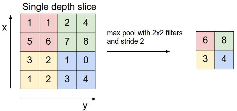
Max pooling ( 2 2) . . ; 2.
. . , , .

, .
N x 28 x 28 x 1. 4 4 16, zero-padding ( padding='SAME' Tensorflow) , N x 28 x 28 x 16. max pooling 2 2 2, N x 14 x 14 x 16. 4 4 32 zero-padding, N x 14 x 14 x 32. max pooling ( ) N x 7 x 7 x 32. . 32 * 7 * 7 625 1568 625, N 625. 625 10 10 .

, . , «» .

, ;
: ;
X, y dropout ;
Cost softmax_cross_entropy_with_logits L2;
— RMSPropOptimizer;
(256), ;
dropout 0.2 convolutional 0.5 . , «» (MNIST) ;
, /. , , , ;

MNIST TF :

 from tensorflow.examples.tutorials.mnist import input_data mnist = input_data.read_data_sets('MNIST_data', one_hot=True) mnist_test_images = mnist.test.images.reshape(-1, 28, 28, 1)

, FNN, - , :

 trX = X_train.reshape(-1, 28, 28, 1) # 28x28x1 teX = X_val.reshape(-1, 28, 28, 1) enc = OneHotEncoder() enc.fit(y.reshape(-1, 1), 10).toarray() # 10x1 trY = enc.fit_transform(y_train.reshape(-1, 1)).toarray() teY = enc.fit_transform(y_val.reshape(-1, 1)).toarray()

CNN FNN, -. - , CNN , . , :

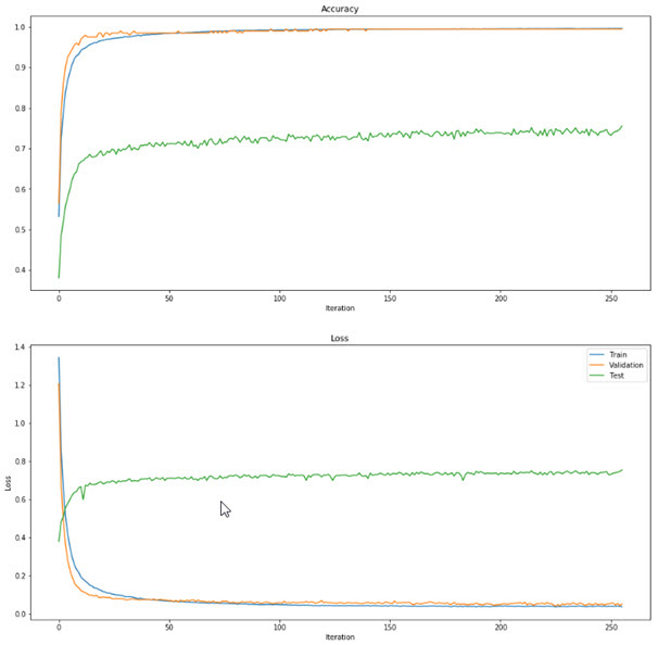
, , ~100 .

CNN , FNN: , 1 , -3 .

CNN

 import numpy as np import boto import boto3 from boto.s3.key import Key from boto.s3.connection import S3Connection import tensorflow as tf import os class CNN(object): """ Convolutional neural network with several levels. The architecture is the following: input - conv - relu - pool - dropout - conv - relu - pool - dropout - fully connected layer - dropout - fully connected layer The outputs of the second fully-connected layer are the scores for each class. """ def __init__(self): """ Initialize the model. Weights are passed into the class. """ self.params = {} def train(self, image, digit): """ Train this neural network. 1 step of gradient descent. Inputs: - X: A numpy array of shape (N, 784) giving training data. - y: A numpy array f shape (N,) giving training labels; y[i] = c means that X[i] has label c, where 0 <= c < C. """ tf.reset_default_graph() init_op = tf.global_variables_initializer() X = tf.placeholder("float", [None, 28, 28, 1]) Y = tf.placeholder("float", [None, 10]) w = tf.get_variable("w", shape=[4, 4, 1, 16], initializer=tf.contrib.layers.xavier_initializer()) b1 = tf.get_variable(name="b1", shape=[16], initializer=tf.zeros_initializer()) w3 = tf.get_variable("w3", shape=[4, 4, 16, 32], initializer=tf.contrib.layers.xavier_initializer()) b3 = tf.get_variable(name="b3", shape=[32], initializer=tf.zeros_initializer()) w4 = tf.get_variable("w4", shape=[32 * 7 * 7, 625], initializer=tf.contrib.layers.xavier_initializer()) b4 = tf.get_variable(name="b4", shape=[625], initializer=tf.zeros_initializer()) w_o = tf.get_variable("w_o", shape=[625, 10], initializer=tf.contrib.layers.xavier_initializer()) b5 = tf.get_variable(name="b5", shape=[10], initializer=tf.zeros_initializer()) p_keep_conv = tf.placeholder("float") p_keep_hidden = tf.placeholder("float") l1a = tf.nn.relu( tf.nn.conv2d( X, w, strides=[1, 1, 1, 1], padding='SAME' ) + b1 ) l1 = tf.nn.max_pool( l1a, ksize=[1, 2, 2, 1], strides=[1, 2, 2, 1], padding='SAME') l1 = tf.nn.dropout(l1, p_keep_conv) l3a = tf.nn.relu( tf.nn.conv2d( l1, w3, strides=[1, 1, 1, 1], padding='SAME' ) + b3 ) l3 = tf.nn.max_pool( l3a, ksize=[1, 2, 2, 1], strides=[1, 2, 2, 1], padding='SAME') #Reshape for matmul l3 = tf.reshape(l3, [-1, w4.get_shape().as_list()[0]]) l3 = tf.nn.dropout(l3, p_keep_conv) l4 = tf.nn.relu(tf.matmul(l3, w4) + b4) l4 = tf.nn.dropout(l4, p_keep_hidden) py_x = tf.matmul(l4, w_o) + b5 # Cost with L2 reg_losses = tf.get_collection(tf.GraphKeys.REGULARIZATION_LOSSES) reg_constant = 0.01 cost = tf.reduce_mean( tf.nn.softmax_cross_entropy_with_logits(logits=py_x, labels=Y) + reg_constant * sum(reg_losses) ) train_op = tf.train.RMSPropOptimizer(0.00001).minimize(cost) predict_op = tf.argmax(py_x, 1) with tf.Session() as sess: # Load weights saver = tf.train.Saver() saver.restore(sess, "./tmp/data-all_2_updated.chkp") trX = image.reshape(-1, 28, 28, 1) trY = np.eye(10)[digit] sess.run(train_op, feed_dict={X: trX, Y: trY, p_keep_conv: 1, p_keep_hidden: 1}) # Save updated weights all_saver = tf.train.Saver() all_saver.save(sess, './tmp/data-all_2_updated.chkp') def predict(self, image, weights='original'): """ Generate prediction for one or several digits. Weights are downloaded from Amazon. Returns: - top_3: a list of 3 top most probable predictions with their probabilities as tuples. """ s3 = boto3.client( 's3', aws_access_key_id=os.environ['AWS_ACCESS_KEY_ID'], aws_secret_access_key=os.environ['AWS_SECRET_ACCESS_KEY'] ) # Choose weights to load if weights == 'original': f = 'data-all_2.chkp' else: f = 'data-all_2_updated.chkp' fn = f + '.meta' s3.download_file('digit_draw_recognize',fn,os.path.join('tmp/',fn)) fn = f + '.index' s3.download_file('digit_draw_recognize',fn,os.path.join('tmp/',fn)) fn = f + '.data-00000-of-00001' s3.download_file('digit_draw_recognize',fn,os.path.join('tmp/',fn)) tf.reset_default_graph() init_op = tf.global_variables_initializer() sess = tf.Session() # Define model architecture X = tf.placeholder("float", [None, 28, 28, 1]) Y = tf.placeholder("float", [None, 10]) w = tf.get_variable("w", shape=[4, 4, 1, 16], initializer=tf.contrib.layers.xavier_initializer()) b1 = tf.get_variable(name="b1", shape=[16], initializer=tf.zeros_initializer()) w3 = tf.get_variable("w3", shape=[4, 4, 16, 32], initializer=tf.contrib.layers.xavier_initializer()) b3 = tf.get_variable(name="b3", shape=[32], initializer=tf.zeros_initializer()) w4 = tf.get_variable("w4", shape=[32 * 7 * 7, 625], initializer=tf.contrib.layers.xavier_initializer()) w_o = tf.get_variable("w_o", shape=[625, 10], initializer=tf.contrib.layers.xavier_initializer()) b4 = tf.get_variable(name="b4", shape=[625], initializer=tf.zeros_initializer()) p_keep_conv = tf.placeholder("float") p_keep_hidden = tf.placeholder("float") b5 = tf.get_variable(name="b5", shape=[10], initializer=tf.zeros_initializer()) l1a = tf.nn.relu( tf.nn.conv2d( X, w, strides=[1, 1, 1, 1], padding='SAME' ) + b1 ) l1 = tf.nn.max_pool( l1a, ksize=[1, 2, 2, 1], strides=[1, 2, 2, 1], padding='SAME') l1 = tf.nn.dropout(l1, p_keep_conv) l3a = tf.nn.relu( tf.nn.conv2d( l1, w3, strides=[1, 1, 1, 1], padding='SAME' ) + b3 ) l3 = tf.nn.max_pool( l3a, ksize=[1, 2, 2, 1], strides=[1, 2, 2, 1], padding='SAME') l3 = tf.reshape(l3, [-1, w4.get_shape().as_list()[0]]) l3 = tf.nn.dropout(l3, p_keep_conv) l4 = tf.nn.relu(tf.matmul(l3, w4) + b4) l4 = tf.nn.dropout(l4, p_keep_hidden) py_x = tf.matmul(l4, w_o) + b5 # Cost with L2 reg_losses = tf.get_collection(tf.GraphKeys.REGULARIZATION_LOSSES) reg_constant = 0.01 cost = tf.reduce_mean( tf.nn.softmax_cross_entropy_with_logits(logits=py_x, labels=Y) + reg_constant * sum(reg_losses) ) train_op = tf.train.RMSPropOptimizer(0.00001).minimize(cost) predict_op = tf.argmax(py_x, 1) probs = tf.nn.softmax(py_x) # Load model and predict saver = tf.train.Saver() saver.restore(sess, "./tmp/" + f) y_pred = sess.run(probs, feed_dict={X: image.reshape(-1, 28, 28, 1), p_keep_conv: 1.0, p_keep_hidden: 1.0}) probs = y_pred # Create list with top3 predictions and their probabilities top_3 = list(zip(np.argsort(probs)[0][::-1][:3], np.round(probs[0][np.argsort(probs)[0][::-1][:3]] * 100, 2))) sess.close() return top_3

learning rate. 0.00001, 100 . , . , .

( ). -, , bootstrap. : html css, js . , , .

. :

main.py , functions.py .

functions.py

 __author__ = 'Artgor' import base64 import os import uuid import random import numpy as np import boto import boto3 from boto.s3.key import Key from boto.s3.connection import S3Connection from codecs import open from PIL import Image from scipy.ndimage.interpolation import rotate, shift from skimage import transform from two_layer_net import FNN from conv_net import CNN class Model(object): def __init__(self): """ Load weights for FNN here. Original weights are loaded from local folder, updated - from Amazon. """ self.params_original = np.load('models/original_weights.npy')[()] self.params = self.load_weights_amazon('updated_weights.npy') def process_image(self, image): """ Processing image for prediction. Saving in temproral folder so that it could be opened by PIL. Cropping and scaling so that the longest side it 20. Then putting it in a center of 28x28 blank image. Returning array of normalized data. """ filename = 'digit' + '__' + str(uuid.uuid1()) + '.jpg' with open('tmp/' + filename, 'wb') as f: f.write(image) img = Image.open('tmp/' + filename) bbox = Image.eval(img, lambda px: 255-px).getbbox() if bbox == None: return None widthlen = bbox[2] - bbox[0] heightlen = bbox[3] - bbox[1] if heightlen > widthlen: widthlen = int(20.0 * widthlen/heightlen) heightlen = 20 else: heightlen = int(20.0 * widthlen/heightlen) widthlen = 20 hstart = int((28 - heightlen) / 2) wstart = int((28 - widthlen) / 2) img_temp = img.crop(bbox).resize((widthlen, heightlen), Image.NEAREST) new_img = Image.new('L', (28,28), 255) new_img.paste(img_temp, (wstart, hstart)) imgdata = list(new_img.getdata()) img_array = np.array([(255.0 - x) / 255.0 for x in imgdata]) return img_array def augment(self, image, label): """ Augmenting image for training. Saving in temporal folder so that it could be opened by PIL. Cropping and scaling so that the longest side it 20. The width and height of the scaled image are used to resize it again so that there would be 4 images with different combinations of weight and height. Then putting it in a center of 28x28 blank image. 12 possible angles are defined and each image is randomly rotated by 6 of these angles. Images converted to arrays and normalized. Returning these arrays and labels. """ filename = 'digit' + '__' + str(uuid.uuid1()) + '.jpg' with open('tmp/' + filename, 'wb') as f: f.write(image) image = Image.open('tmp/' + filename) ims_add = [] labs_add = [] angles = np.arange(-30, 30, 5) bbox = Image.eval(image, lambda px: 255-px).getbbox() widthlen = bbox[2] - bbox[0] heightlen = bbox[3] - bbox[1] if heightlen > widthlen: widthlen = int(20.0 * widthlen/heightlen) heightlen = 20 else: heightlen = int(20.0 * widthlen/heightlen) widthlen = 20 hstart = int((28 - heightlen) / 2) wstart = int((28 - widthlen) / 2) for i in [min(widthlen, heightlen), max(widthlen, heightlen)]: for j in [min(widthlen, heightlen), max(widthlen, heightlen)]: resized_img = image.crop(bbox).resize((i, j), Image.NEAREST) resized_image = Image.new('L', (28,28), 255) resized_image.paste(resized_img, (wstart, hstart)) angles_ = random.sample(set(angles), 6) for angle in angles_: transformed_image = transform.rotate(np.array(resized_image), angle, cval=255, preserve_range=True).astype(np.uint8) labs_add.append(int(label)) img_temp = Image.fromarray(np.uint8(transformed_image)) imgdata = list(img_temp.getdata()) normalized_img = [(255.0 - x) / 255.0 for x in imgdata] ims_add.append(normalized_img) image_array = np.array(ims_add) label_array = np.array(labs_add) return image_array, label_array def load_weights_amazon(self, filename): """ Load weights from Amazon. This is npy. file, which needs to be read with np.load. """ s3 = boto3.client( 's3', aws_access_key_id=os.environ['AWS_ACCESS_KEY_ID'], aws_secret_access_key=os.environ['AWS_SECRET_ACCESS_KEY'] ) s3.download_file('digit_draw_recognize', filename, os.path.join('tmp/', filename)) return np.load(os.path.join('tmp/', filename))[()] def save_weights_amazon(self, filename, file): """ Save weights to Amazon. """ REGION_HOST = 's3-external-1.amazonaws.com' conn = S3Connection(os.environ['AWS_ACCESS_KEY_ID'], os.environ['AWS_SECRET_ACCESS_KEY'], host=REGION_HOST) bucket = conn.get_bucket('digit_draw_recognize') k = Key(bucket) k.key = filename k.set_contents_from_filename('tmp/' + filename) return ('Weights saved') def save_image(self, drawn_digit, image): """ Save image on Amazon. Only existing files can be uploaded, so the image is saved in a temporary folder. """ filename = 'digit' + str(drawn_digit) + '__' + \ str(uuid.uuid1()) + '.jpg' with open('tmp/' + filename, 'wb') as f: f.write(image) REGION_HOST = 's3-external-1.amazonaws.com' conn = S3Connection(os.environ['AWS_ACCESS_KEY_ID'], os.environ['AWS_SECRET_ACCESS_KEY'], host=REGION_HOST) bucket = conn.get_bucket('digit_draw_recognize') k = Key(bucket) k.key = filename k.set_contents_from_filename('tmp/' + filename) return ('Image saved successfully with the \ name {0}'.format(filename)) def predict(self, image): """ Predicting image. If nothing is drawn, returns a message; otherwise 4 models are initialized and they make predictions. They return a list of tuples with 3 top predictions and their probabilities. These lists are sent to "select_answer" method to select the best answer. Also tuples are converted into strings for easier processing in JS. The answer and lists with predictions and probabilities are returned. """ img_array = self.process_image(image) if img_array is None: return "Can't predict, when nothing is drawn" net = FNN(self.params) net_original = FNN(self.params_original) cnn = CNN() cnn_original = CNN() top_3 = net.predict_single(img_array) top_3_original = net_original.predict_single(img_array) top_3_cnn = cnn.predict(img_array, weights='updated') top_3_cnn_original = cnn_original.predict(img_array, weights='original') answer, top_3, top_3_original, top_3_cnn, top_3_cnn_original = self.select_answer(top_3, top_3_original, top_3_cnn, top_3_cnn_original) answers_dict = {'answer': str(answer), 'fnn_t': top_3, 'fnn': top_3_original, 'cnn_t': top_3_cnn, 'cnn': top_3_cnn_original} return answers_dict def train(self, image, digit): """ Models are trained. Weights on Amazon are updated. """ r = self.save_image(digit, image) print(r) # Start models and train them net = FNN(self.params) X, y = self.augment(image, digit) net.train(X, y) cnn = CNN() cnn.train(X, y) # Save updated weights. np.save('tmp/updated_weights.npy', net.params) response = self.save_weights_amazon( 'updated_weights.npy', './tmp/updated_weights.npy' ) response = self.save_weights_amazon( 'data-all_2_updated.chkp.meta', './tmp/data-all_2_updated.chkp' ) response = self.save_weights_amazon( 'data-all_2_updated.chkp.index', './tmp/data-all_2_updated.chkp' ) response = self.save_weights_amazon( 'data-all_2_updated.chkp.data-00000-of-00001', './tmp/data-all_2_updated.chkp' ) return response def select_answer(self,top_3,top_3_original,top_3_cnn,top_3_cnn_original): """ Selects best answer from all. In fact only from the trained models, as they are considered to be better than untrained. """ answer = '' # If answers are the same, show this answer. if int(top_3[0][0]) == int(top_3_cnn[0][0]): answer = str(top_3[0][0]) # If answers' probabilities are low, show fail message. elif int(top_3[0][1]) < 50 and int(top_3_cnn[0][1]) < 50: answer = "Can't recognize this as a digit" # Otherwise show answer with highest probability elif int(top_3[0][0]) != int(top_3_cnn[0][0]): if int(top_3[0][1]) > int(top_3_cnn[0][1]): answer = str(top_3[0][0]) else: answer = str(top_3_cnn[0][0]) top_3 = ['{0} ({1})%'.format(i[0], i[1]) for i in top_3] top_3_original = ['{0} ({1})%'.format(i[0], i[1] for i in top_3_original] top_3_cnn = ['{} ({:2.4})%'.format(i[0], i[1]) for i in top_3_cnn] top_3_cnn_original = ['{} ({:2.4})%'.format(i[0], i[1]) for i in top_3_cnn_original] return answer, top_3, top_3_original, top_3_cnn, top_3_cnn_original

«» , . FNN — , init , .

, tmp ( , ). , Amazon. , load_weights_amazon

Amazon : , ( , , os.environ['AWS_ACCESS_KEY_ID'] , , : aws_access_key_id=os.environ['AWS_ACCESS_KEY_ID'] ). bucket , .

Tensorflow , . , Tensorflow .

JS Python predict . , — , . , , . JS, , .

4 . FNN , .

CNN , — . .

4 . ? select_answer . FNN CNN: , ; 50%, , ; , , , ( ). , ( ) , JS. JS.

JS , — .

:

( ) Python;
( ) , ;
train, 1 ;
;

. :

canvas — , ;
«Predict» — , , ;
«Allow to use the drawn digit for model training» — , . / ;
«Yes» — , ( );
«No» — , ( );
«Clear» — canvas ;
/ ;

JS / : document.getElementById().style.display «none» «block».

, , , .

. , , - . bootstrap , . , . mozilla . , : ontouchstart, ontouchmove, ontouchend. , , ;
- . MNIST , , . … , Heroku , , ;
: , . : CNN . … , . , , , . .
, : , . , . : Models . Flask. python , ;

プロジェクトの開始

23 « » . . , , ( ). , , , , « ». .

— . 2 : , ; mozilla . , , , .
— , / ( , , ), , «» .

: . , , 2,5 ( , ). … :

~ , ( slack ODS) . , , .

«-». , , . — - google quickdraw , . — SVM . , , — ( ), ;
. : -;
— ;
/ ;
/ . , «Yes» «No»;
PC — , ;

おわりに

. . . . . , , data science , .

オンラインで再トレーニングして手書きの数字を認識するためのプロジェクトを作成する方法。初心者向けではないガイド

私について少し

アイデアの起源

本体

プロジェクト計画

データ収集

サイトの最初のバージョンの作成（データ収集用）

フラスコについて簡単に

プロジェクト構造

HTMLとJS

フラスコと画像保存

Amazon S3の統合

ヘロク

モデルの画像処理

画像増強

FNN

FNN

CNN

プロジェクトの開始

おわりに

More articles:

オンラインで再トレーニングして手書きの数字を認識するためのプロジェクトを作成する方法。 初心者向けではないガイド

私について少し

アイデアの起源

本体

プロジェクト計画

データ収集

サイトの最初のバージョンの作成（データ収集用）

フラスコについて簡単に

プロジェクト構造

HTMLとJS

フラスコと画像保存

Amazon S3の統合

ヘロク

モデルの画像処理

画像増強

FNN

FNN

CNN

プロジェクトの開始

おわりに

More articles:

オンラインで再トレーニングして手書きの数字を認識するためのプロジェクトを作成する方法。初心者向けではないガイド