この記事では、R
ggpubr 、
cowplot、および
gridExtraパッケージで利用可能なヘルパー関数を使用して、1つ以上の図にいくつかの
ggplotグラフを組み合わせる方法を順を追って説明し
ます 。 また、結果のグラフをファイルにエクスポートする方法についても説明します。
行または列を並べ替える
ggpubrパッケージを使用する
ネストされた
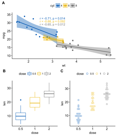
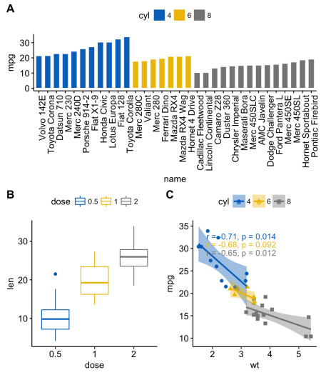
ggarrange()関数を使用して、行または列のグラフの配置を変更します。
たとえば、次のコードは次のことを行います。
- 散布図(sp)は最初の行にあり、2列を占有します
- 散布図(bxp)および散布図(dp)は、2行目と2つの異なる列を占有します
ggarrange(sp, # ggarrange(bxp, dp, ncol = 2, labels = c("B", "C")), # nrow = 2, labels = "A" # )
カウプロットパッケージの使用
次の関数の組み合わせ[
カウプロットパッケージから]を使用して、指定されたサイズの特定の場所にグラフィックを配置できます:
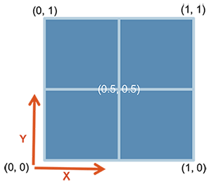
ggdraw() + draw_plot() + draw_plot_label()ggdraw()。 空のキャンバスを初期化します。
ggdraw()
デフォルトでは、座標が0から1に変わり、ポイント(0、0)はキャンバスの左下隅にあることに注意してください(下の図を参照)。
draw_plot()。 キャンバス上のどこかにグラフがあります:
draw_plot(plot, x = 0, y = 0, width = 1, height = 1)
plot :配置するグラフ(ggplot2またはgtable)x, y :グラフの左下隅のx / y座標width, height :グラフの幅と高さ
draw_plot_label()。 グラフの右上隅にラベルを追加します
関連付けられた座標を持つラベルベクトルを使用できます。
draw_plot_label(label, x = 0, y = 1, size = 16, ...)
label : labelベクトルx, y :それぞれのラベルのx / y座標を持つベクトルsize :ラベルのフォントサイズ
たとえば、この方法では、サイズの異なる複数のグラフを特定の場所に結合できます。
library("cowplot") ggdraw() + draw_plot(bxp, x = 0, y = .5, width = .5, height = .5) + draw_plot(dp, x = .5, y = .5, width = .5, height = .5) + draw_plot(bp, x = 0, y = 0, width = 1, height = 0.5) + draw_plot_label(label = c("A", "B", "C"), size = 15, x = c(0, 0.5, 0), y = c(1, 1, 0.5))

gridExtraパッケージを使用する
[
gridExtra ]の
arrangeGrop()関数は、行または列のグラフの配置を変更するのに役立ちます。
たとえば、次のコードは次のことを行います。
- 散布図(sp)は最初の行にあり、2列を占有します
- 散布図(bxp)および散布図(dp)は2行目と2つの異なる列を占有します
library("gridExtra") grid.arrange(sp, # arrangeGrob(bxp, dp, ncol = 2),# nrow = 2) #
grid.arrange()関数では、
layout_matrix引数を使用して複雑なグラフ
layout_matrixを作成することもでき
layout_matrix 。
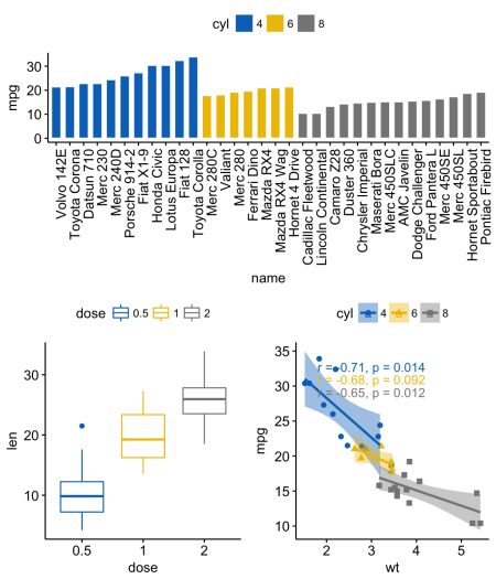
以下のコードでは、
layout_matrixは2x2マトリックス(2行2列)です。 最初の行はすべて単位で、最初のグラフは2列を占めます。 2行目にはグラフ2と3が含まれ、それぞれが独自の列を占めています。
grid.arrange(bp, # bxp, sp, # ncol = 2, nrow = 2, layout_matrix = rbind(c(1,1), c(2,3)))
また、ヘルパー関数
draw_plot_label() [
カウプロット ]を使用して、
grid.arrange()関数の出力に注釈を追加することもできます。
grid.arrange()または
arrangeGrob()関数
grid.arrange() arrangeGrob()型)の
grid.arrange()注釈を簡単に追加するに
grid.arrange()最初に
as_ggplot()関数[
ggpubr ]を使用してそれらをggplot型に変換する必要があります。 その後、
draw_plot_label()関数を[to
cowplot ]に適用できます。
library("gridExtra") library("cowplot") # arrangeGrob # gtable (gt) gt <- arrangeGrob(bp, # bxp, sp, # ncol = 2, nrow = 2, layout_matrix = rbind(c(1,1), c(2,3))) # p <- as_ggplot(gt) + # ggplot draw_plot_label(label = c("A", "B", "C"), size = 15, x = c(0, 0, 0.5), y = c(1, 0.5, 0.5)) # p
上記のコードでは、
arrangeGrob()代わりに、
grid.arrange()を使用し
arrangeGrob() 。 これら2つの関数の主な違いは、
grid.arrange()が順序付きグラフを自動的に表示することです。 グラフを描画する前に注釈をグラフに追加したかったため、この場合は、
arrangeGrob()関数を使用することをお
arrangeGrob()します。
グリッドパッケージの使用
gridパッケージでは、
grid.layout()関数を使用して、グラフの複雑な相互配置を指定できます。 また、領域またはスコープを指定する
viewport()ヘルパー関数も提供します。
print()関数は、特定の領域にチャートを配置するために使用されます。
手順は次のように説明できます。
- グラフの作成:p1、p2、p3、...
grid.newpage()関数を使用して新しいページに移動します- 2X2レイアウトの作成-列数= 2; 行数= 2
- スコープの設定:グラフィックデバイス上の長方形の領域
- スコープ内のグラフを印刷する
library(grid) # grid.newpage() # : nrow = 3, ncol = 2 pushViewport(viewport(layout = grid.layout(nrow = 3, ncol = 2))) # define_region <- function(row, col){ viewport(layout.pos.row = row, layout.pos.col = col) } # print(sp, vp = define_region(row = 1, col = 1:2)) # print(bxp, vp = define_region(row = 2, col = 1)) print(dp, vp = define_region(row = 2, col = 2)) print(bp + rremove("x.text"), vp = define_region(row = 3, col = 1:2))

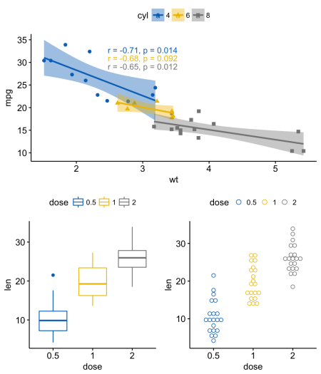
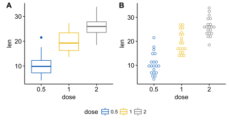
結合されたggplotグラフィックスに共通の凡例を使用する
いくつかの順序付けられたグラフに共通の凡例を指定するには、
ggarrange()関数[
ggpubr内 ]を次の引数とともに使用できます。
common.legend = TRUE :共通の凡例を作成しますlegend : legendの位置を設定します。 許可される値はc(「上」、「下」、「左」、「右」)のいずれかです。
ggarrange(bxp, dp, labels = c("A", "B"), common.legend = TRUE, legend = "bottom")
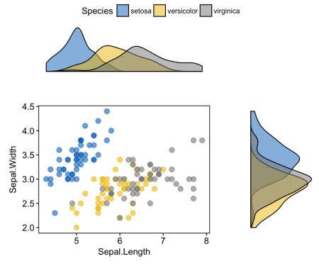
無条件の分布密度プロットを含む散布図
# , ("Species") sp <- ggscatter(iris, x = "Sepal.Length", y = "Sepal.Width", color = "Species", palette = "jco", size = 3, alpha = 0.6)+ border() # x ( ) y ( ) xplot <- ggdensity(iris, "Sepal.Length", fill = "Species", palette = "jco") yplot <- ggdensity(iris, "Sepal.Width", fill = "Species", palette = "jco")+ rotate() # yplot <- yplot + clean_theme() xplot <- xplot + clean_theme() # ggarrange(xplot, NULL, sp, yplot, ncol = 2, nrow = 2, align = "hv", widths = c(2, 1), heights = c(1, 2), common.legend = TRUE)
次のパートでは:
- テーブル、テキスト、ggplot2-graphicsを混在させる
- グラフィック要素をggplotに追加します(テーブル、散布図、背景画像)
- 複数のページにグラフィックを配置する
- ネストされた相対位置
- チャートエクスポート